Check out this repo to see how we’ve applied it.
While building our home garden controller, Kindbot, the chief objective was to maintain ideal environmental conditions. Plants thrive under stable temperatures which is often a challenge for those running powerful grow lights in a small space.
Let’s consider a generic microcontroller connected to a environmetal sensor breakout. Furthermore, let’s assume you can control a heating/cooling appliance via the microcontroller’s GPIO pins or through communication with a smart plug over the LAN.
A space will tend to run either cooler or warmer than your desired set point. Let’s assume without loss of generality that temperatures tend to run warmer than our set point but we can control an air conditioner/fan.
After turning on the air conditioner, it takes a moment for cool air to diffuse and affect the ambient temperature. We’ll begin by choosing the length of time that we will run a cooling cycle, also called the duty cycle.
We should choose a time length interval based on how quickly we expect an appreciable temperature change to occur. In other words, if temperature changes marginally over 1 minute, its reasonable to choose a longer time interval, perhaps 3 minutes. This helps to avoid unneccesary computations while reducing the mechanical wear on appliances.
Industry Standard Approach
Often, thermostats will use PID control to regulate duty cycles. Binary decisions (appliance on/off) are made after applying a threshold to the sum of three terms: one Proportional to the controller error, another proportional to the accumulated (Integrated) error over successive time steps, and finally a term proportional to the rate of change (Derivative) of this error.
Unfortunately, tuning the PID controller takes some experimentation to get the best performance. Additionally, when the temperature dynamics change, perhaps due to design changes in the space or seasonal effects, PID control performance may degrade.
Generalizing Temperature Control Models
Thermal systems can be strongly impacted by ambient conditions but, for our smart thermostat, we want a controller robust to external influences. Further, we do not want to specialize PID control to perform well in one temperature control problem, only to find our controller fails to perform well in a setup with different temperature dynamics.
For example, given a heat source, smaller spaces will tend to concentrate heat and maintain warmer temps for the same level of ventilation or cooling. Since we want an easy, accessible smart thermostat to work with minimal setup/configuration, we need to develop a controller which can adapt to changes in the ambient environment while generalizing to setups with different dynamics.
Adaptive Control
While there are algorithms that can be used to autotune a PID controller, deciding when to retune becomes a new problem. Instead of imposing so many assumptions in our temperature control task, we explore reframing the temperature control problem in terms of a game that an AI agent plays to accumulate points.
State Information
To determine whether running an air conditioner for the next duty cycle is necessary, we periodically evaluate recent actions and environmental sensor data using recent temperature and humidity. We can incorporate this with information on the time of day or year.
Then our temperature control agent will decide at each discrete time step whether or not to activate the cooling appliance for the duration of the subsequent duty cycle.
Close Enough
Our temperature sensor will have limited precision and so, for the purposes of evaluating our model, we will regard temperatures with a small difference from the target set point as essentially equivalent.
Penalties & Rewards
If at the beginning of a cycle, the temperature lies outside of this epsilon band around the set point, we will deduct points from the running game play point total. To penalize big errors more severely, let’s choose the number of points to subtract in a way proportional to the magnitude of the temperature difference between temperature readings and our target set point.
Alternatively, to reward our temperature control agent for maintaining temps near the set point, we add many points. We chose something like 10 points since we expect the order of error to be lower than ten degrees.
We apply a discount rate on rewards to model the temporal dependence of the current state on previous state-action decisions. We chose a discount rate of 0.5 since its powers vanish quickly in order to model a weak dependences of current state on previous states and actions.
Learning a Policy
We need to determine a policy which will use the available environmental state information as input and return a chosen action like ‘turn on the ac’ as output.
Neural networks can be great function approximators and we want to learn weights of a neural network to approximate our policy function. In this way, we will be able to apply the neural network to our state information to make decisions.
Since we have no way to model arbitrary temperature dynamics, we must learn our policy after making empirical observations on how actions impact temperatures. Our policy function will produce a distribution over available actions for a given input state. Then our agent will sample from this distribution with a strong preference for making the optimal choice while allowing some exploration. After many observations, we expect patterns to emerge which help to associate optimal action choices with given environmental state information.
Putting it Together
We choose a duty cycle length of 3 minutes since temperature changes rather slowly. We’ll regard temperatures within two degrees farenheit of our set point as equivalent for the purposes of the reward function. When we observe temperatures within this epsilon band, the agent is rewarded with 10 points. Otherwise, the agent is penalized by losing points, the number of which is proportional to the difference in current temperature and the target set point temperature.
We will learn a policy function to associate state information like recent temps and actions, along with time of day or year information to a distribution over available actions: ‘turn the ac on/off’.
We will use a neural network to approximate the policy function and we will select an action by sampling from the distribution to allow for some exploration while maintaining near optimal performance.
Ultimately, we improve our policy by backpropagating information gained after each episode. More precisely, we adjust model weights in a way proportional to the total reward accumulated over an episode of several subsequent time steps. This will effectively reinforce neural network connections that lead to high value actions while reducing the tendency to select actions that are associated with strong penalties.
Putting these ideas into code, we have the reward function:
def reward_function(temp):
    temp_diff = np.abs(temp - setpoint)
    if temp_diff < 2:
        return 10
    else:
        return -temp_diff
The policy function is approximated using the following simple network:
X = tf.placeholder(tf.float32, shape=[None, n_inputs])
hidden = tf.layers.dense(X, n_hidden, activation=tf.nn.elu, kernel_initializer=initializer)
logits = tf.layers.dense(hidden, n_outputs)
outputs = tf.nn.sigmoid(logits)  # probability of action 0 (off)
Our input dimension was 21 after concatenating recent actions as well as temperature and humidity information along with a numerical representation of the hour of day and month of the year.
We sample the network output to select the next action with:
p_on_and_off = tf.concat(axis=1, values=[outputs, 1 - outputs])
action = tf.multinomial(tf.log(p_on_and_off), num_samples=1)
To perform backpropagation using our Monte Carlo estimates after episodes of successive time steps, we need to get the gradients so we can apply a reasonable discount rate to model the time dependence between the current state and recent action choices.
y = 1. - tf.to_float(action)
cross_entropy = tf.nn.sigmoid_cross_entropy_with_logits(labels=y, logits=logits)
optimizer = tf.train.AdamOptimizer(learning_rate)
grads_and_vars = optimizer.compute_gradients(cross_entropy)
gradients = [grad for grad, variable in grads_and_vars]
gradient_placeholders = []
grads_and_vars_feed = []
for grad, variable in grads_and_vars:
    gradient_placeholder = tf.placeholder(tf.float32, shape=grad.get_shape())
    gradient_placeholders.append(gradient_placeholder)
    grads_and_vars_feed.append((gradient_placeholder, variable))
training_op = optimizer.apply_gradients(grads_and_vars_feed)
By introducing a few helper functions for sqlite3 logging as well as controlling a TP-Link smart plug, we can build a script which runs in an online manner to learn the AC control policy to maintain temperatures near our ideal set point. Check out this repo for an example application.
Conclusion
Allowing the model to train, our agent learns to perform temperature control by optimizing for accumulated points over many successive episodes, collecting points when temps are near the set point while deducting points when temps fall out of target range.
In our experiments, this model was more flexible than PID control while offering greater stability by reduced overshooting and oscillation when temperatures increase at the beginning of the day as lamp heat accumulates in the space.
Since our controller has no knowledge that what it controls is an AC, by symmetry, we could use a heater for spaces that tend to run cooler than our target set point.
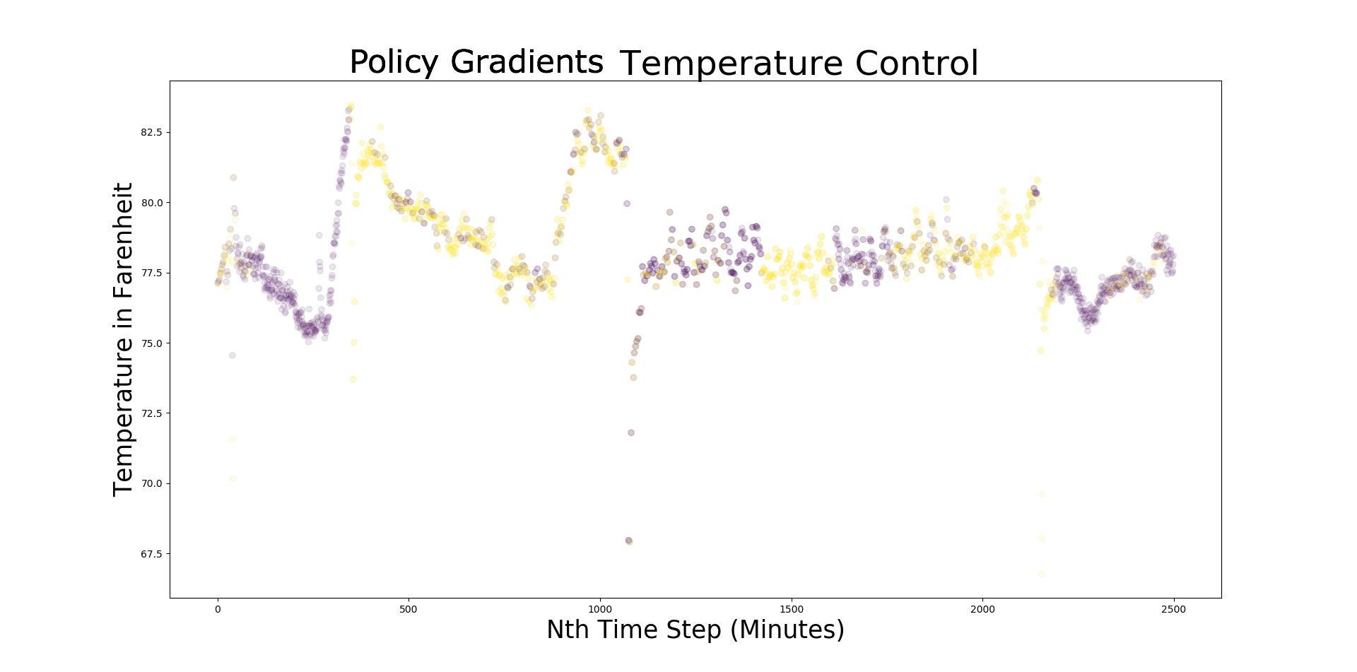
In the plot above, we show several days worth of temperature control targeting the setpoint of 77 degrees Farenheit by controling a fan with a smart plug. This took place in a space that would otherwise exceed 100 degrees under a powerful High Intensity Discharge lamp as a heat source. Yellow markers indicate a duty cycle with the fan running while purple markers designate duty cycles with the fan off.