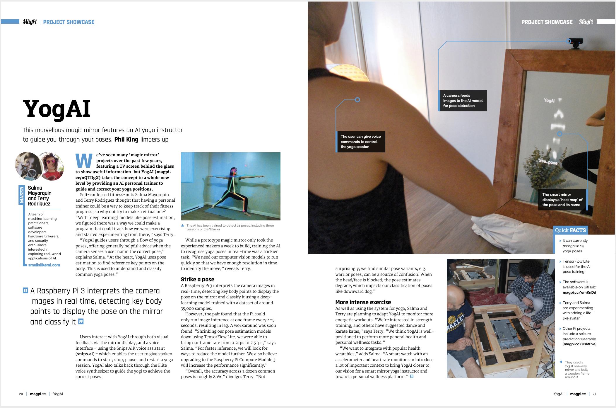
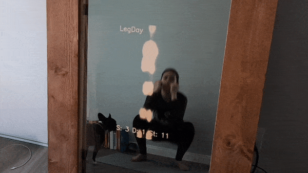
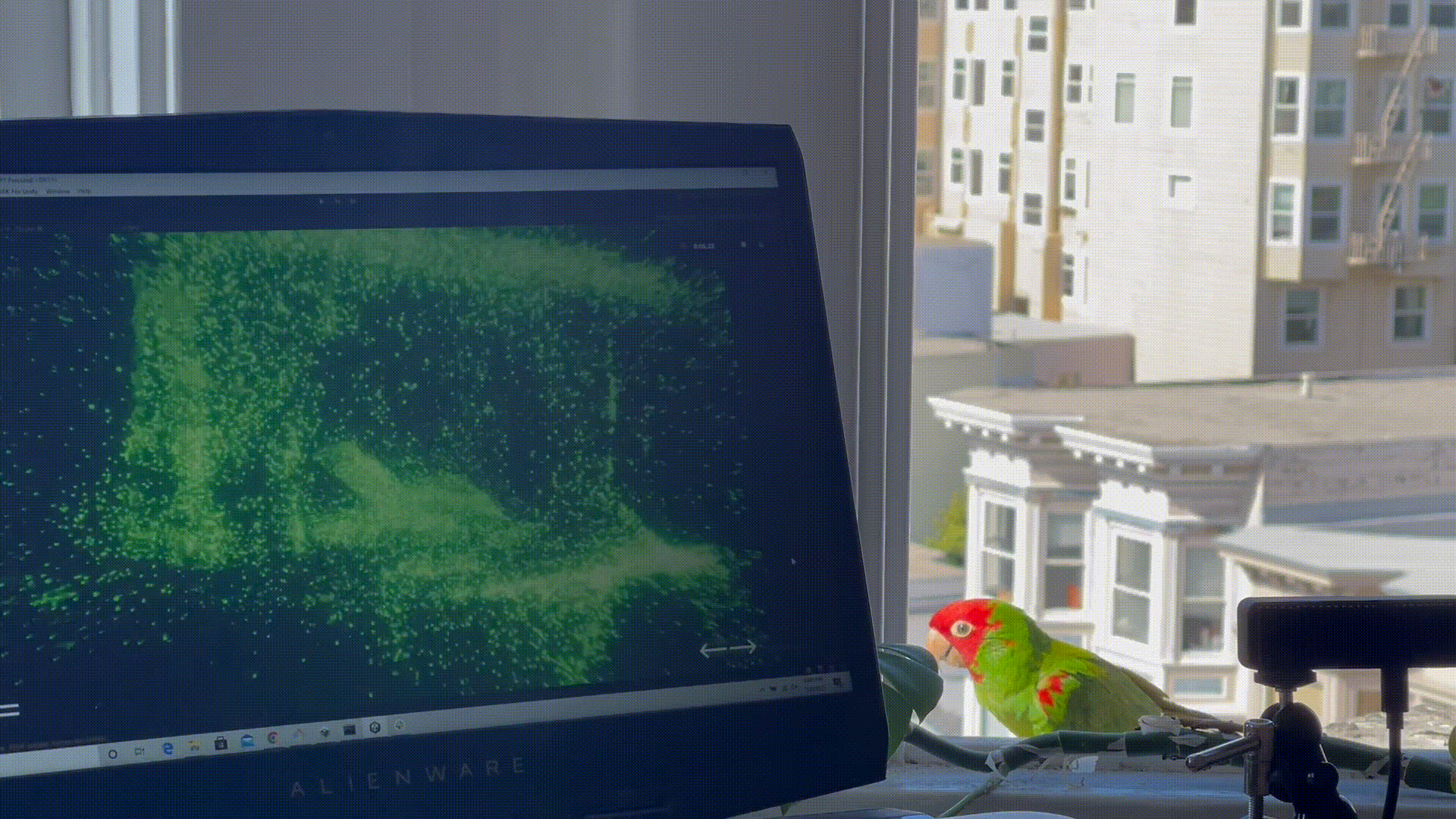
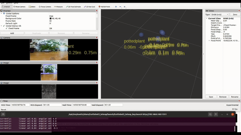
Some of our earliest work applying ML to video was done in the context of prototyping IoT products like YogAI.
A couple years ago, we described a more generalized pipeline called ActionAI.
ActionAI was designed to streamline prototyping IoT products using lightweight activity recognition pipelines on devices like NVIDIA’s Jetson Nano or the Coral Dev Board.
Since then, NVIDIA has introduced action recognition modules into their Deepstream SDK. They model a classifier using 3D convolutional kernels over the space-time volume of normalized regions of interest, batched over a k-window in time.
In fact, many SOTA results in video understanding and activity recognition employ 3D convolution or larger multi-stream network architectures.
More recently, researchers adapt Vision Transformers (ViT) to this task and some work has progressed from the task of recognition to anticipation.
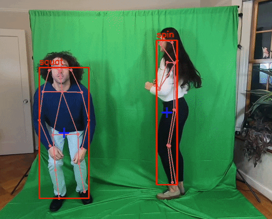
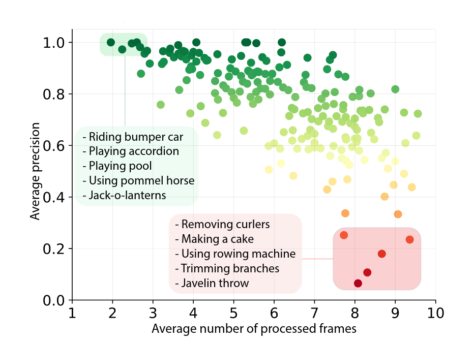
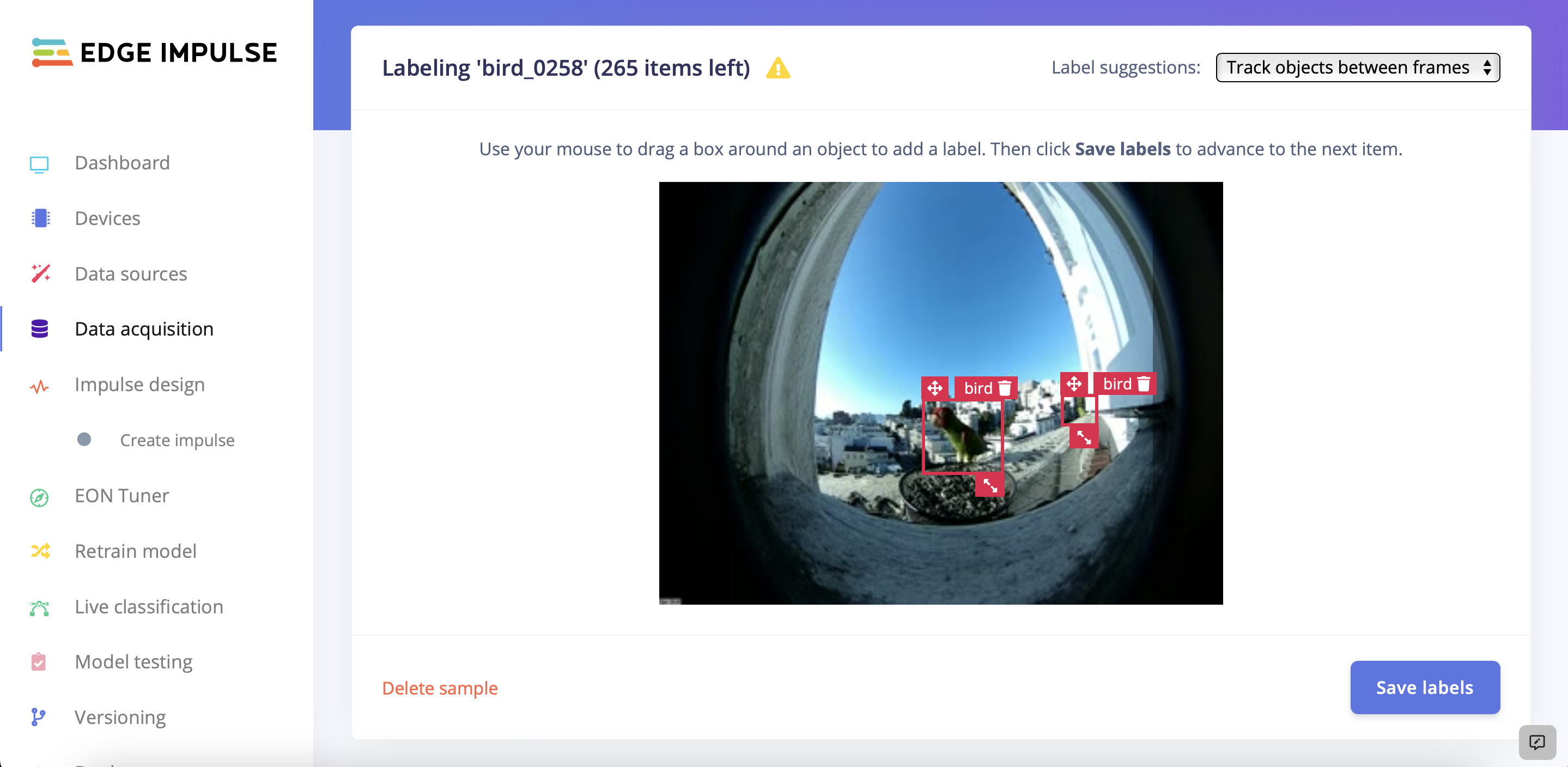
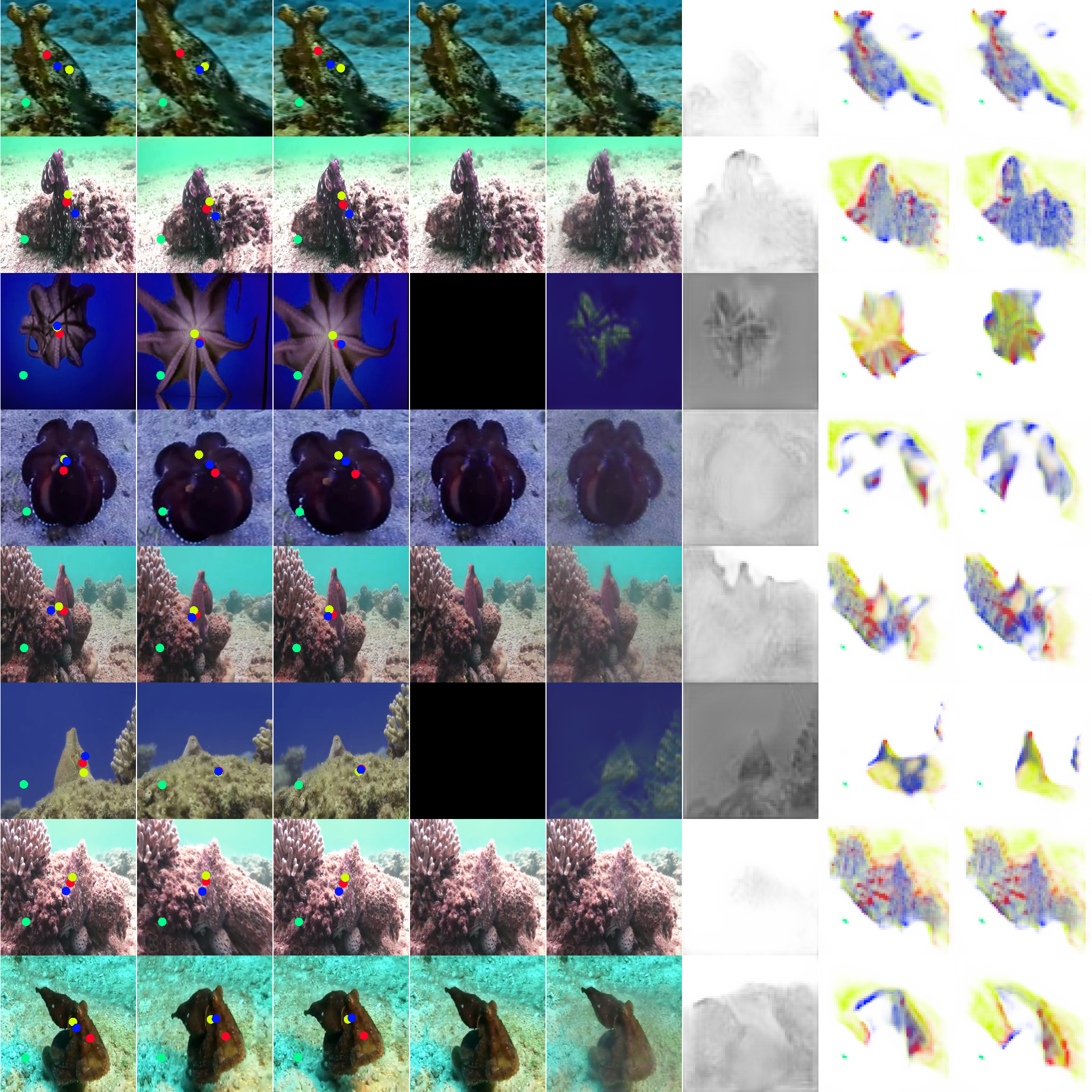
In prototyping IoT products featuring human-computer interactions with ActionAI, we found the rich and highly localized context of pose estimation model inference results helpful.
Applying Keypoint Detectors as fixed feature extractors also helped to project our high-bandwidth image input to low-dimensional features. From there, we can optimize sequential models to classify motion thereby limiting the capacity of our model to overfit to visual characteristics of people in motion.
Over this timeline, we have also been exploring related applications of human-centric video analytics pipelines for the purposes of deepfake detection:
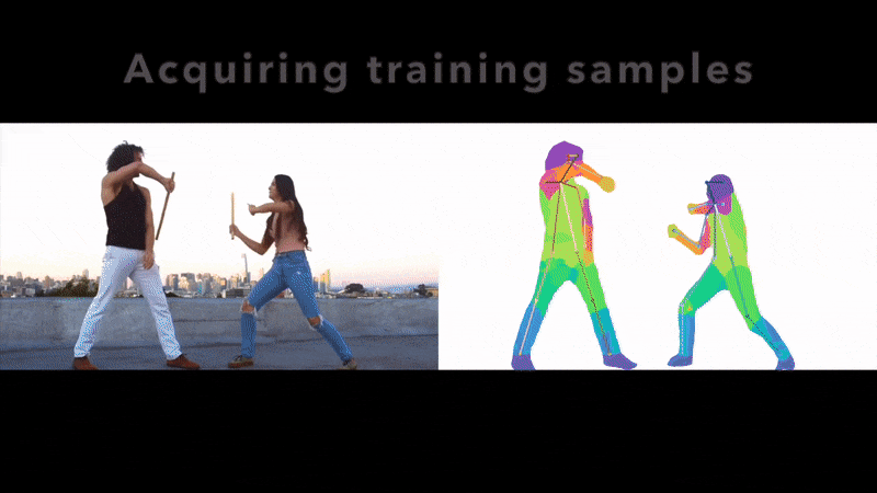
As well as motion transfer, here with two-person transfer of a fight scene using kali sticks:
We’ve explored adapting ActionAI to the use of hand keypoints, face keypoints, and face embeddings but we have also been keen to generalize beyond these readily available models.
To those ends, we have been exploring first-order motion models (FOMM) and its related corpus of work. In our experiments generating content, we were impressed by the ability to apply these models across domain.
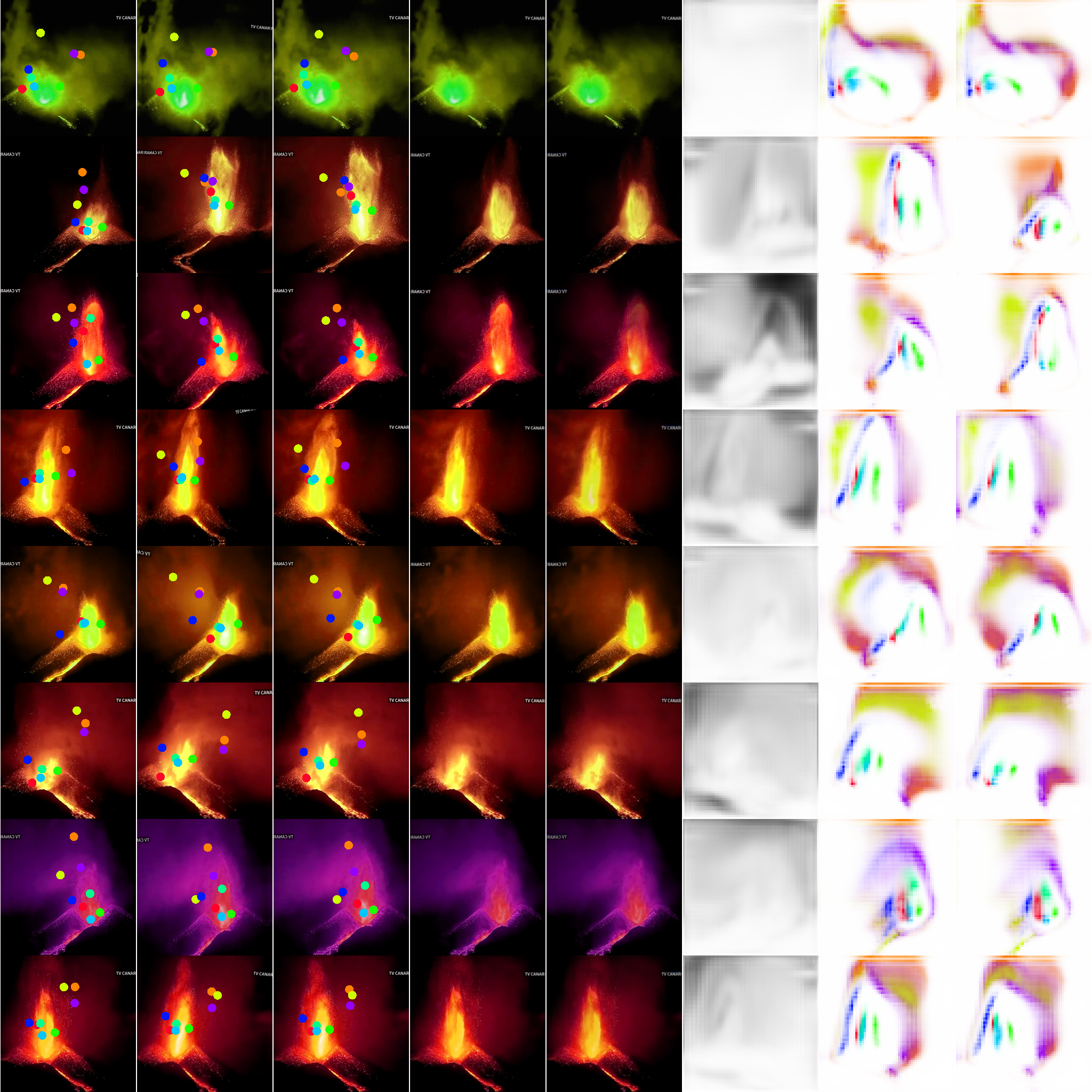
This impressive success in self-supervised learning of keypoint detectors for arbitrary objects led us to ask “What else could we do with few-shot video understanding by generalizing ActionAI pipeline ideas through the use of these keypoint detectors?”
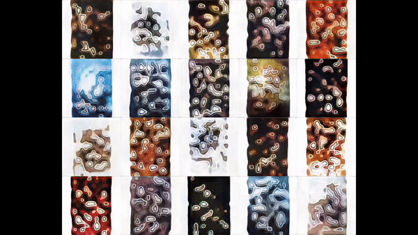
With a sample youtube video, we can characterize the motion of many object categories using self-supervised learning. Here we drive a synthesized image which happens to look like a volcanic eruption via articulated animation.
For many animated objects of interest, a mode of activity can be characterized by little more than motion and frequency over gross spatial and temporal scales with respect to camera’s field-of-view. We appreciate the potential to accelerate science and especially the analysis of complex biological behaviors under controlled studies by bootstrapping from relatively little training data.
Inferring modes of activity this way can be insufficient for video understanding, where the context of object-object interactions becomes relevant. Nonetheless, for many practical applications, a structured pipeline using detection & tracking will facilitate the extraction of additional cues through secondary models with prediction cascades.
Along those lines, we were recently introduced to the work in MovieGraphs, which endows richly annotated video with graph structure to perform video understanding. In application like film analysis, we may expect the expensive feature extraction is justified by recognizing its amortization over a lifetime of repeated consumption for human entertainment.
We believe graphs can be efficient in modeling complex interactions over space and time through pipelines like ActionAI, but we also want to emphasize real-time performance on resource-limited edge hardware.
Looking back at ActionAI, we realize it has been our most popular project and facilitated many related applications for us. But ActionAI has potential for much more than a repo documenting this collection of early AIoT prototypes.
In fact, this project has helped us gain attention and partnerships with the biggest groups in tech as they adopt related techniques in video understanding and perception.
But we believe ActionAI has the potential to accelerate these use cases in the same way projects like face_recognition and dlib have served users of those libraries.
As discussed above, we have many directions to consider but we aim to lean into lightweight and robust video pipelines. For starters, we might consider additional reductions to the training pipeline for these region predictors.
Consider joining the ActionAI Gitter where we can make this conversation dynamic!
title: “Alexa, where are my keys?”
date: 2018-11-05T18:00:00-00:00
tags: [‘raspberry pi’, ‘ble’, ‘edge’]
draft: false
Alexa works well for information retrieval tasks and controlling devices on your wireless home networks. We want to use the home network to track our valuables or keys. We’ll hack cheap bluetooth low energy beacons for the network range and battery longevity and build a smart application so that Alexa knows where we left the keys.
Hacking Bluetooth beacons
We’ll start by exploring what we can do with cheap bluetooth beacons.
A set of 3 beacons can be purchased for less than $15 on Amazon. These are very hackable and even iOS/Android compatible. This adafruit tutorial on reverse engineering smart lights helped us control the beacons. Start by turning on the beacon scan for the device address by running:
sudo hcitool lescan
Find & copy the address labeled with the name ‘iTag,’ then run:
sudo gatttool -I
Connect to the device interactively by running:
connect AA:BB:CC:DD:EE:FF
You should see something like this:
Running ‘char-desc’ followed by the service handle as above, we find UUIDs which we look up by referencing the gatt characteristic specifications and service specifications. For more on these services, check this out. Inspecting traffic with Wireshark, we find that 0100111000000001 triggers the alarm and guess that 0000111000000001 turns it off. Now we have the simple python function:
This function will make the bluetooth tag beep to aid the user in finding the valuables when they are nearby.
Making key finding smarter
With idle computers and raspberry pis spread throughout the house, we query the bluetooth beacon for the RSSI signal strength.
Taking readings from multiple machines, we use RSSI signal strength as a proxy for physical distance. We need to figure out how to use this to compute the most likely part of the house to find the beacon.
We use a simple, fast machine learning algorithm of gradient boosting machines called XGBoost. To get training data for our classifier, we run a crontab job every 2 minutes to query RSSI while we move the beacon to different parts of the house. After some time, we build a jsonl file of RSSI signal strengths from various machines for multiple rooms.
For example, put the beacon in different locations like: ‘Bedroom’, ‘Bathroom’, ‘Kitchen’, ‘Living Area’ to build up a couple dozen readings for each zone. Then we can train a classifier to predict the location based on RSSI signal strengths returned from the various computers around the house.
Loading the tuple of RSSI signal strengths into an array called train with the associated array of string location labels called label, we can train a classifier and use pickle to persist the model as below:
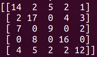
To get a sense of how well the model performs, we inspect the confusion matrix. This will help us determine if we should gather more readings or add another computer to the list. Confusion matrix indices correspond to our alphabetically sorted labels list rows correspond to actual labels with colums corresponding to predicted labels in a 20% hold out validation data set. We can iterate until we are satisfied with the results, aiming for most counts concentrated along the main diagonal of the confusion matrix.
The xgboost implementation of gradient boosting will handle the missing data which we’ll find with timed out readings. XGBoost also trains quickly, taking only seconds. We use python pickle to store the trained model. We load the pickled model into our alexa retrievr application and when we ask alexa for our keys, the most our model runs inference on the most recent RSSI readings on file.
We create a skill that will be linked to a local server. Then we configure our server to take any action we’d like, in this case, provide an approximation for where the keys might be located and make the Bluetooth beacon beep.
Flask provides a simple and easy to use python library to serve an application. Using flask-ask, we can configure the server to communicate with our Alexa skill we’ll build later. Well serve the application with Ngrok, which will give us an https link we’ll need for our Alexa skill. First we built the application with the simplest functionality: to make our BLE beacon beep when triggered and predict its most likely location.
Let’s break down this app for a moment. The retrievr() function is tied to the “findkeys” intent using the @ask.intent() decorator. This means that when our Alexa skill recognizes the “findkeys” intent is being triggered, it will execute whatever is in the retriver() function. This function first executes a script “sound_alarm.py” which contains the function we wrote earlier while hacking the beacons. Then it calls the function guess_locate() defined below. This function calls the loc_predict() on the model we’ve pickled earlier. It reads the most recent logs and taking the last 5 readings, returns a prediction of which room the ble is located. This text string is finally fed to the flask-ask statement() function that will make your Alexa respond with the location.
Remember, you can find all this code in our repo. Let’s build the Alexa skill to tie into this flask-ask app.
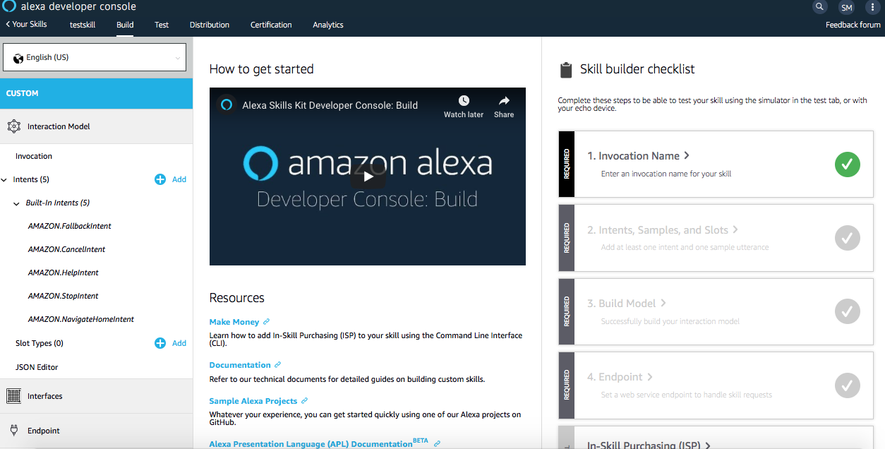
To build the Alexa skill, navigate to the Amazon developer dashboard and log in. Click on Alexa to get to the Alexa Skill kit. You should be greeted by your Alexa Developer Console.
Create a new skill by clicking the Create Skill button. You should see a screen like the one below. Name your skill and continue to the next step.
When prompted to choose a template, choose the Start from scratch option. Continue on to see this next screen:
You’ll work down the skill builder checklist on the right hand side of the screen. Go to Invocation Name and choose a name to invoke your skill. Moving on to the Intents tab on the left hand side, this is where we’ll provide an intent schema to tie our flask-ask app to an Alexa skill. Make sure you’re on the JSON Editor screen of this tab. Edit the JSON file to add a “findkeys” intent.
{"name": "findkeys",
"samples": ["Find my keys", "Where are my keys", "Help me find my keys", "I lost my keys"]},
It should look something like this:
Make sure to save each step as you go! Skip over to the Endpoint tab. Select the https radio button. It’ll prompt you to provide a link to your app. Run the app.py script and in a separate terminal window, run ngrok to generate an https link:
#Go to the dir where you installed ngrok
./ngrok http 5000
Copy and paste the https link generated in each text box. For the SSL Certificate type, select the middle option that describes a wildcard certificate. Skip to Intent History, and after saving, click the Build Model button to build you skill model. This may take a few minutes, so go grab some coffee.
After saving your work, look to the top bar options:
Navigate to the Test tab to test your skill in the Developer Console. On the left hand side, you’ll see a chat interface where you can ask your Alexa skill “Help me find my keys”.
If you want to test on a physical device, use these instructions.
Putting it all Together
Having a model to approximate the last location of the keys, we can add it to the application to improve the statement returned by Alexa.
We created a new function called guess_locate() which takes a file with the latest recorded rssi signal strengths. It’ll then run the samples against our pickled xgboost model and return the most likely location string. This location will be returned when Alexa is prompted. Since establishing a connection to a beacon can take a few seconds, we run a separate process calling that function in sound_alarm.py.
Wrapping all this into an Alexa skill, we can now find our keys anywhere in the house much faster.
title: “Applying GAN Latent Factors for Image Retrieval”
date: 2021-02-26T12:16:34-08:00
tags: [“GANs”, “deep learning”]
draft: false
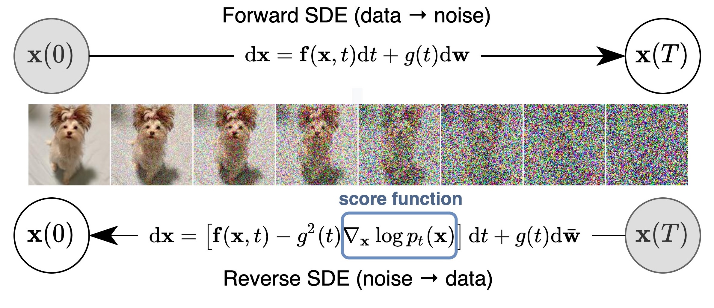
GANs consistently achieve state of the art performance in image generation by learning the distribution of an image corpus.
The newest models often use explicit mechanisms to learn factored representations for images which can be help provide faceted image retrieval, capable of conditioning output on key attributes.
In this post, we explore applying StyleGAN2 embeddings in image retrieval tasks.
StyleGAN2
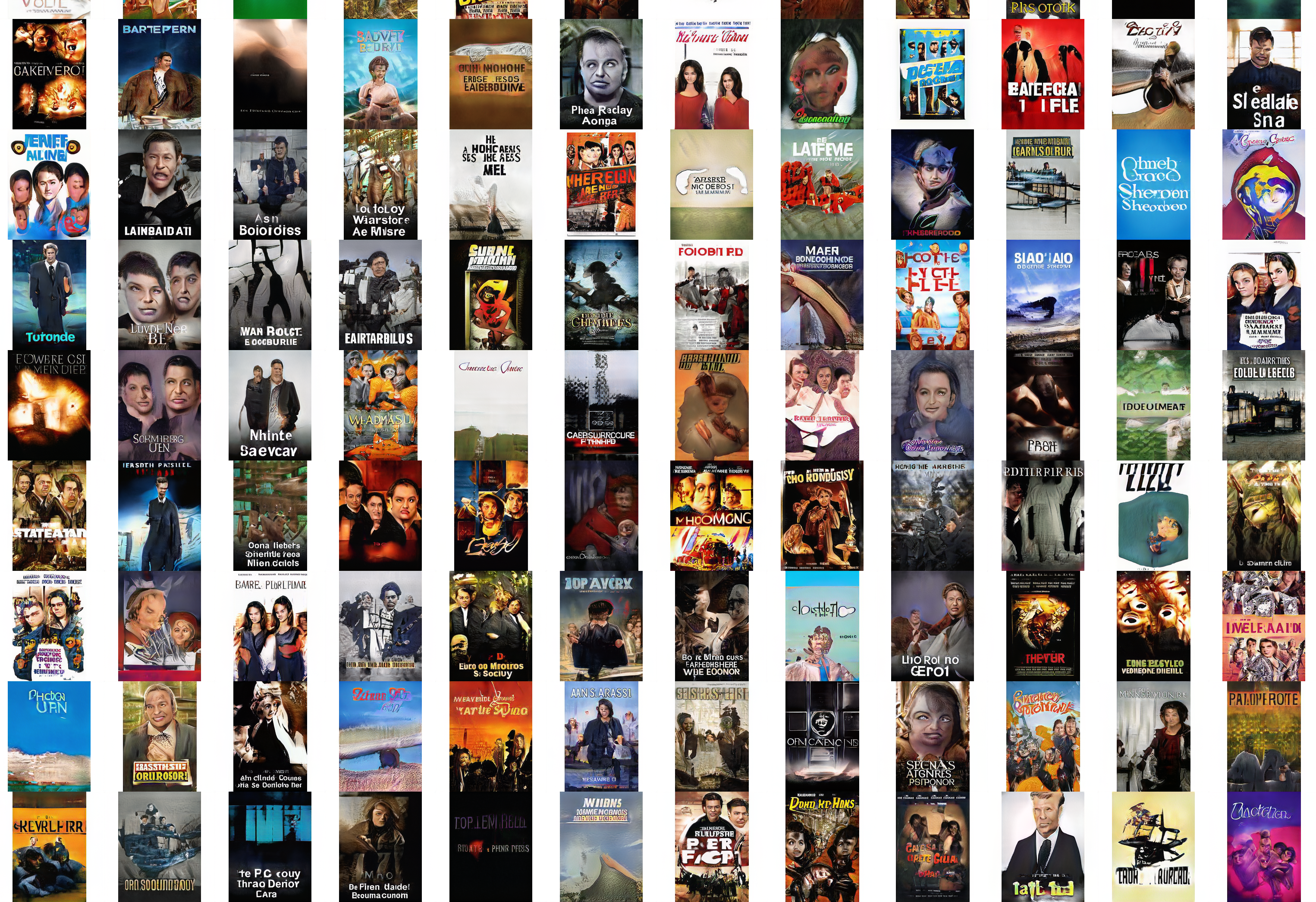
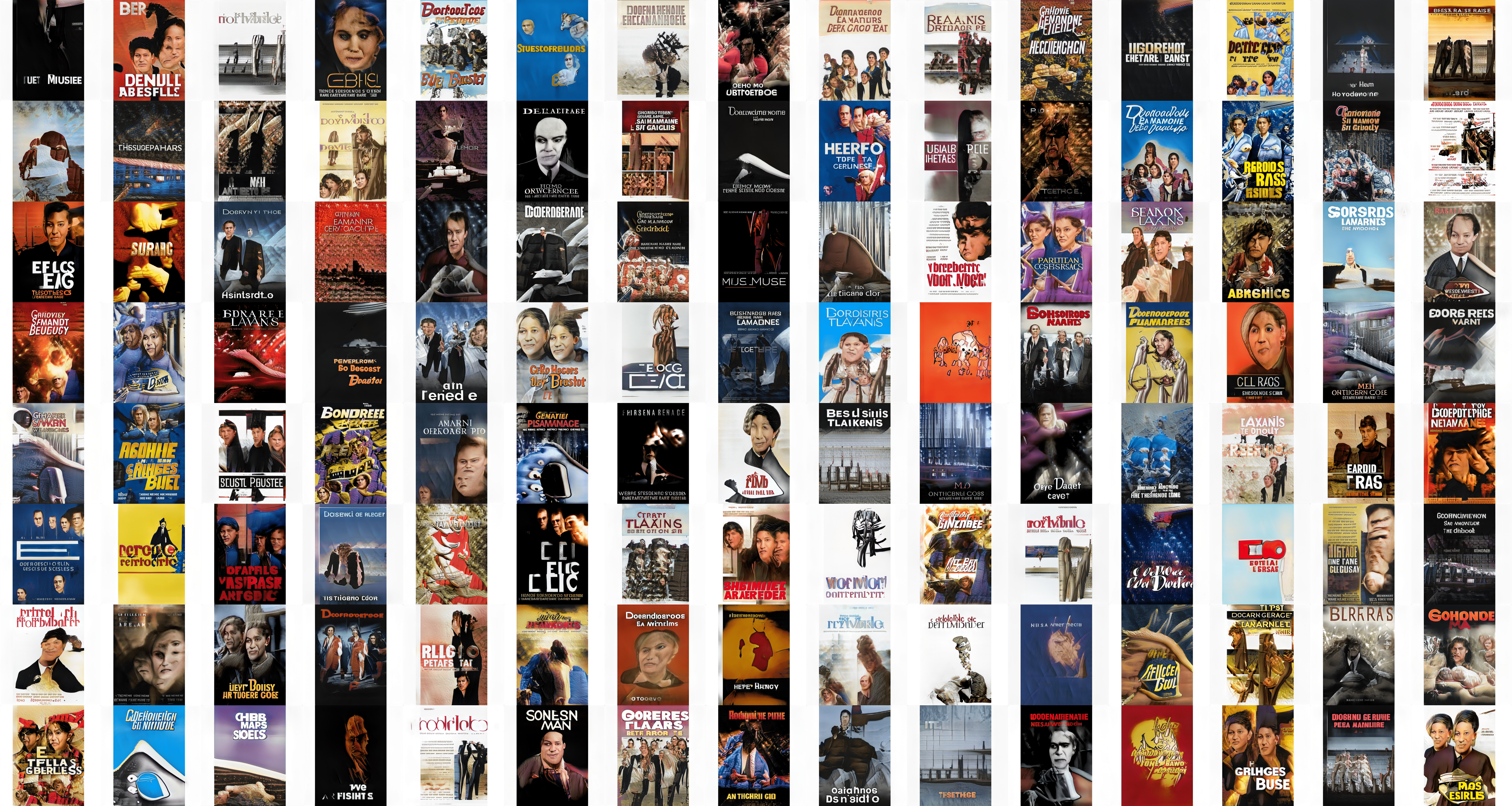
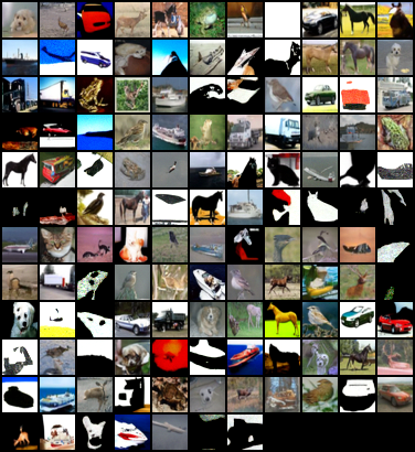
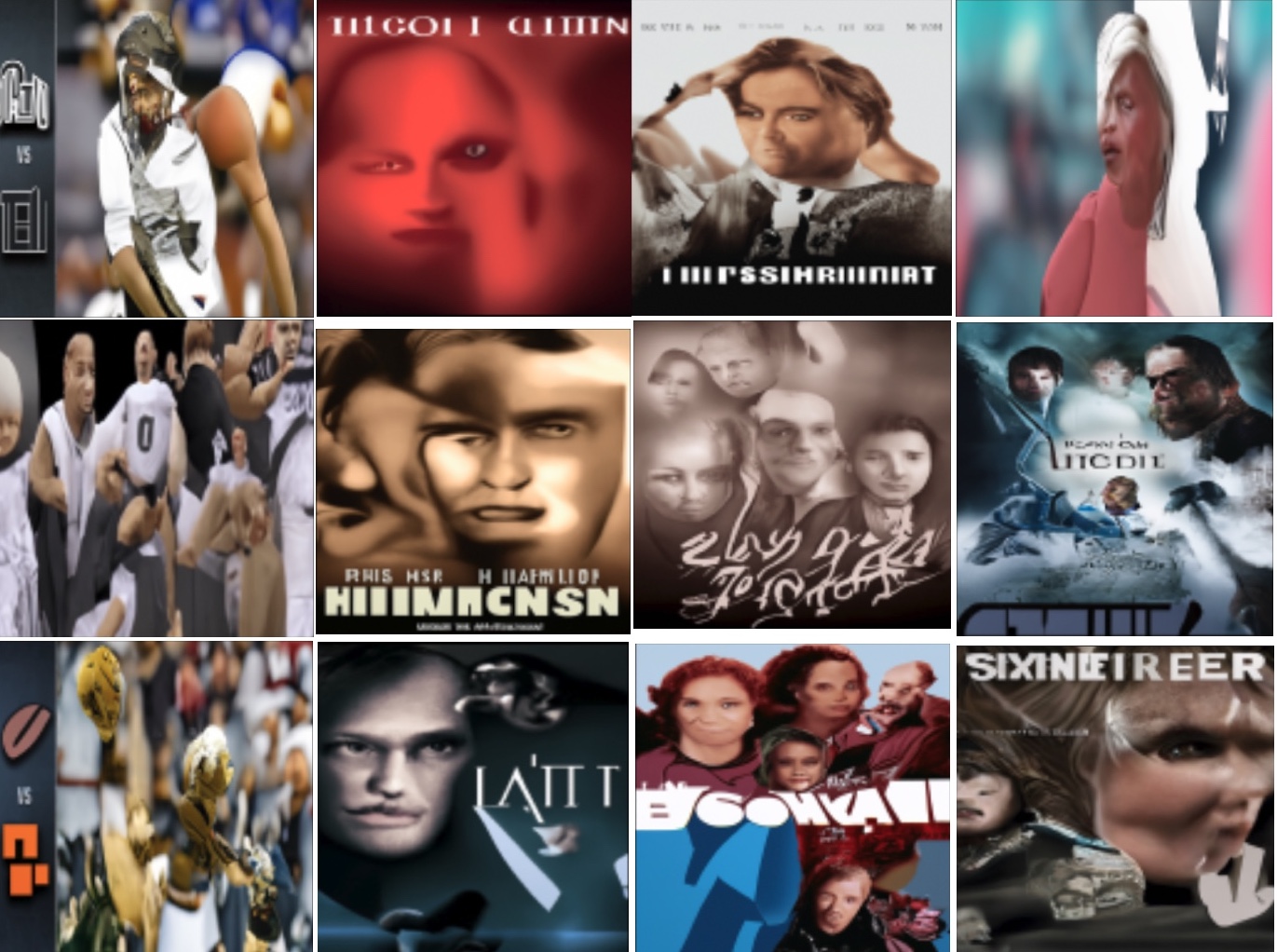
To begin, we train a StyleGAN2 model to generate theatrical posters from our image corpus.
After training the model for 3 weeks on nearly a million images, we finally begin to observe plausible posters.
See a sample realistic enough to fool Google Image search.
A trained StyleGAN2 model can even mix styles between sample images, crossing color palette and textures.
As a byproduct of training our generative model, we obtain methods to produce latent factor representations for each training sample.
Here, we see that StyleGAN2 learns an embedding for each training sample which has some of the characteristics we look for to apply in the image retrieval task.
This approach has the added advantage of not requiring labels to train a model. Despite this, training and generating latent factors was costly! Even if we consider this cost amoritized over an application’s lifecycle, these models are prone to mode collapse and thus poor embeddings.
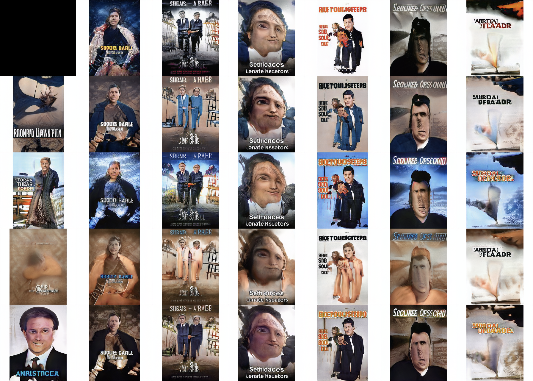
StyleGAN2-ADA
A recent update to StyleGAN2 uses an adaptive test-time image augmentation scheme to stabilize training with fewer samples. Importantly, this is done in such a way that augmentations do not leak into the generated samples.
This variant can reach similar results to the original StyleGAN2 model with an order of magnitude fewer images in a shorter amount of time. It is also possible to train a new model from a checkpoint generated from the original StyleGAN2 architecture.
Besides requiring fewer images, this model allows for class-conditional training, meaning we can introduce genre labels for additional context.
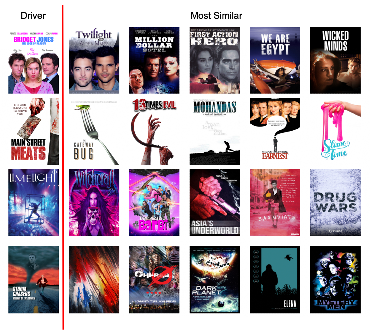
After fine-tuning from our previous checkpoint file on our image corpus for one day, our generated posters look promising.
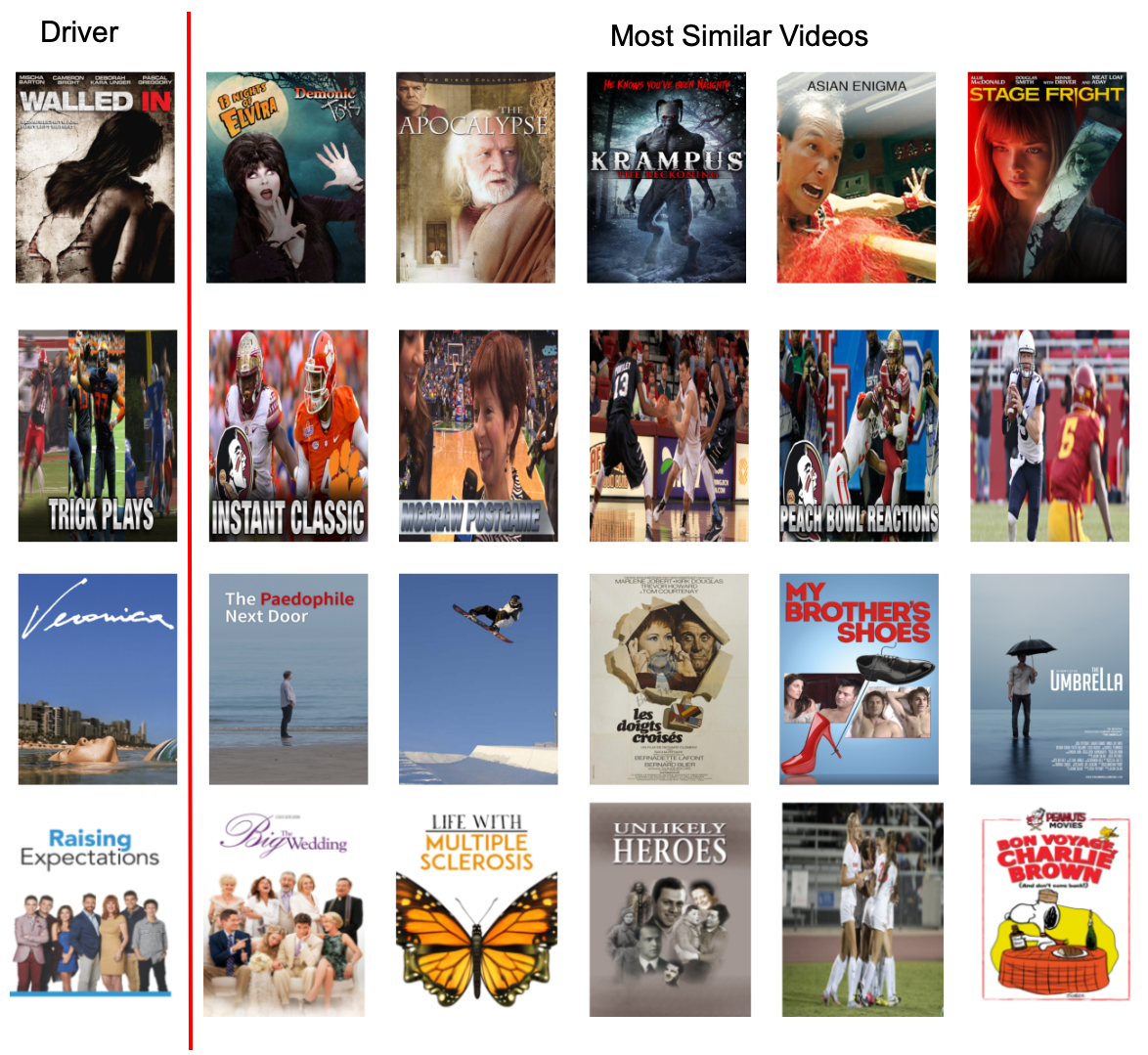
Comparing the most similar posters for a handful of random sample posters, we can see that this new model can capture semantic, color, and texture features like its predecessor in a fraction of the time.
Conclusion
StyleGAN latent factors can effectively capture visual similarity in posters. However, based on some manual review, we consider the metric learning embeddings to be more semantically cohesive.
If an overfit discriminator is the bottleneck for improving the GAN performance, we might consider augmenting the image dataset with additional secondary genre labels.
Overall, this method could be useful where labels are sparse or non-existent for a large image corpus and the recent developments with StyleGAN2 in particular make this approach more tractable. Also, the use of the FID-score provides some helpful proxy for comparing training runs which may also guide metric learning evaluations.
describe approach of selecting samples using search
piles of positive and negative samples for each individual code
describe RNN approach to make a binary classier model for every code
Advances in NLP - BERT
The introduction of BERT by Google was groundbreaking for the NLP space when it was released in 2018.
BERT is based on the Transformer architecture, making it a “bidirectional” model thus allowing it to learn the context of a word based on all its surrounding text. This structure is also easy to parallelize while training since it does not need to process input sequentially.
In practice, BERT expanded the ability to use transfer learning for a variety of tasks. It has the capacity to be pretrained on a large corpus of unlabeled data and the flexibility to add additional layers for finetuning and generating output.
Training an Multi-Label Classifier with BERT
Similar to what how we made our movie poster embeddings, we’ll train a multi-label classifier using a BERT model pretrained on medical text. Once trained, we can use the model to output possible HCC codes corresponding to a member’s medical records.
Using the HuggingFace transformer library makes it easy to preprocess our data and get a model training. Besides providing a nice abstraction for various model architectures, they also have a large repository of pretrained NLP models. For this use case, we used the BioRedditBERT model from the University of Cambridge Language Technology Lab.
Before we start building our model from the pretrained base, we need to process the training data. Using a tokenizer, we transform the text into arrays of numeric tokens representing each word in the sample. This along with an array representing HCC codes identified for each document will be our training data. We store the training samples into tfrecords for efficient training.
title: “Bitrate Optimization using Spark and FFmpeg”
date: 2021-04-13T08:25:39-07:00
tags: [“spark”, “video”, “optimization”]
draft: false
Streaming video is quickly occupying the lion’s share of digital content consumed by users of many applications. At the same time more users are streaming from mobile devices, screen sizes are also increasing while consumers expect high-quality video without lag or distortion artifacts. This frames an engineering challenge to optimize the way video is streamed for consumers across a multitude of hardware platforms.
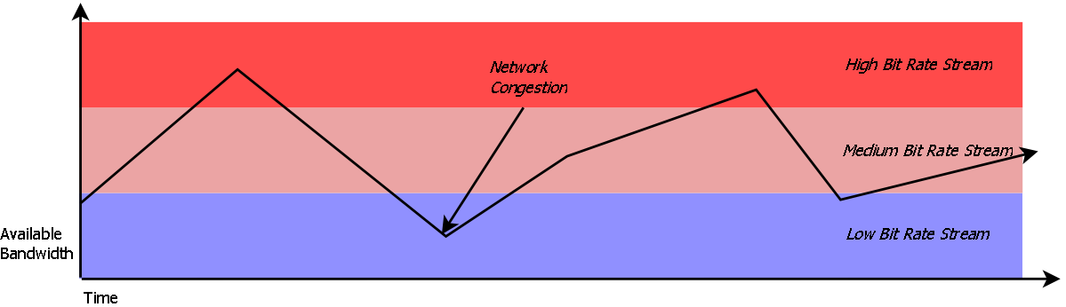
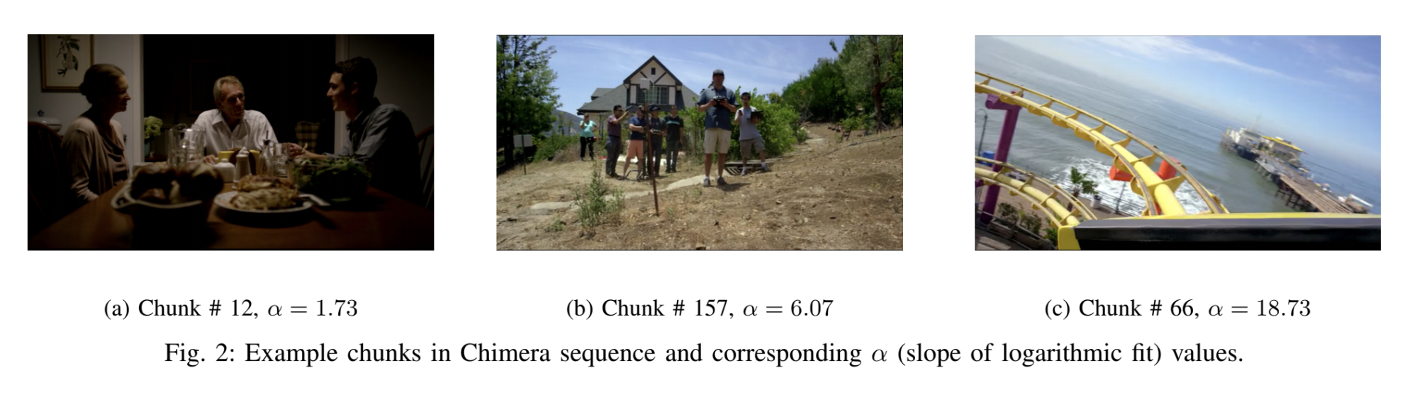
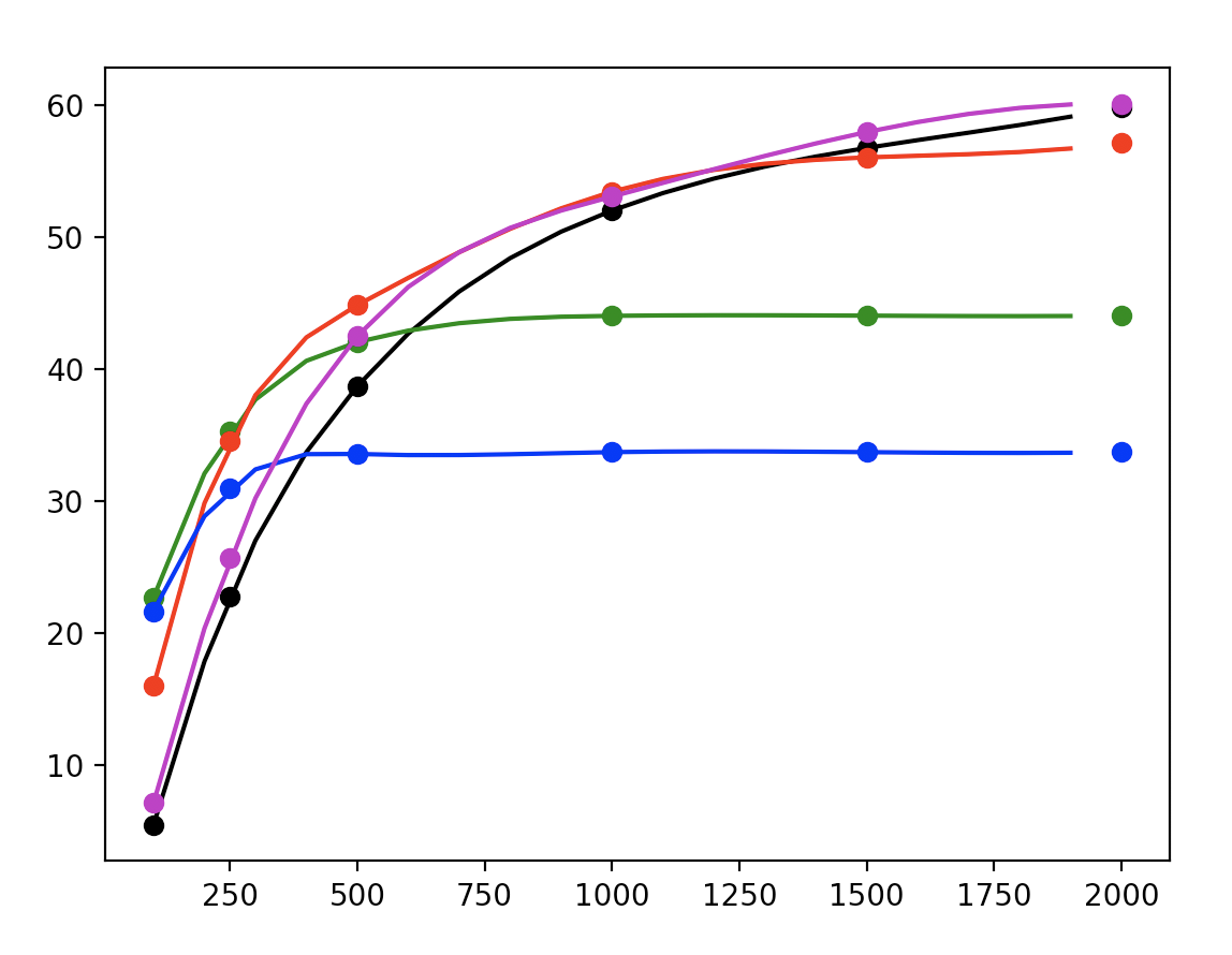
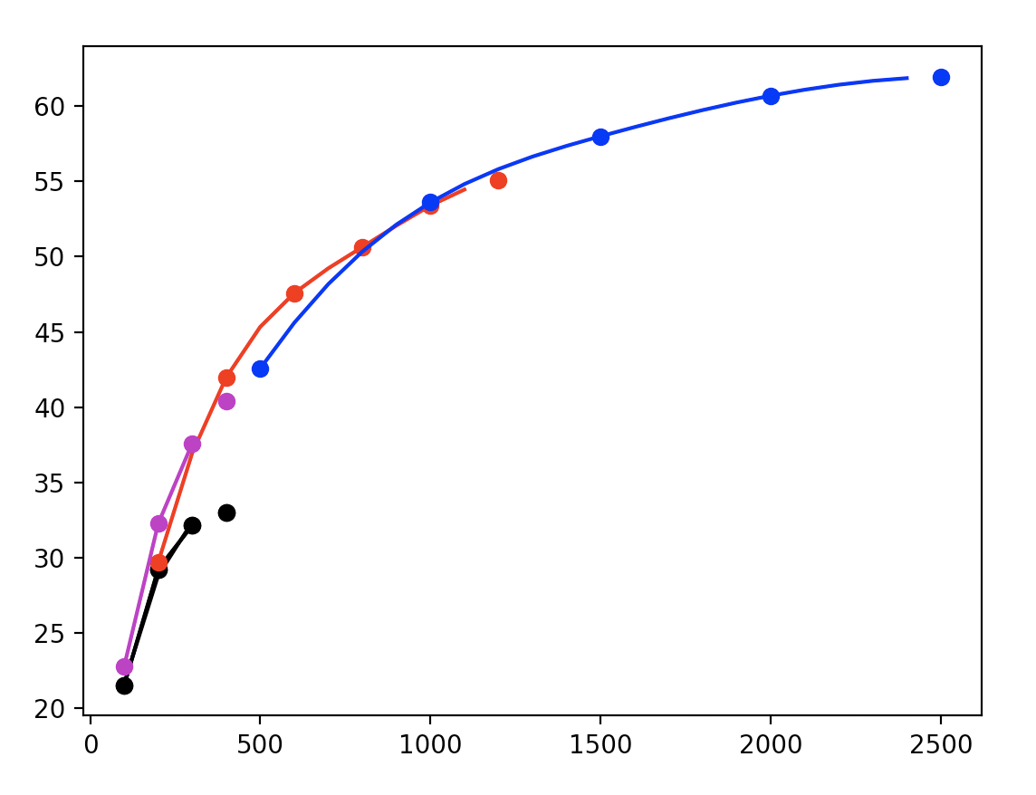
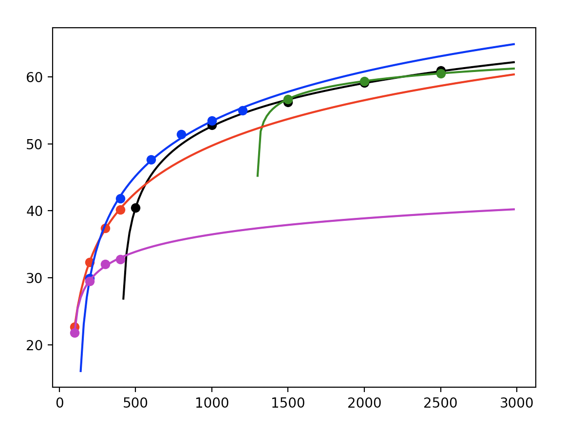
Video streaming sites typically employ adaptive bitrate encoding, whereby video is chunked into groups of pictures (GOPs) and encoded at various bitrate-resolution combinations, allowing client devices to switch dynamically to accommodate changing network conditions.
The perceived quality of streaming video can vary depending on bitrate and resolution. To minimize distortion, we seek the video encoding which optimizes for perceived quality.
Generally, we measure signal distortion using PSNR with respect to a reference but metrics like SSIM, MOS and VMAF are also popular choices for video.
Improved streaming experience is core to experience for Netflix users and their engineers found that encodings can be specialized to each title. Using shot detection, they make additional chunk-level optimizations.
For content which will be streamed by many users, the extra work can be justified by tremendous impact!
Taking this further, researchers found additional gains using content-aware encodings. For example, simple animated images are easy to compress compared to fast-motion & spatially complex video sequences.
Groups like Facebook and Twitter have also employed these kinds of optimizations to scale streaming services to mobile users more efficiently.
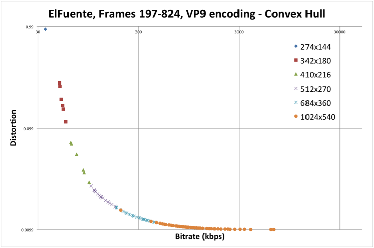
However, encoding video at various bitrate/resolution combinations to compute VMAF against a reference video is computationally very expensive. Additionally, convex hull optimization is required to determine find the best bitrate ladder.
With a naive grid search, we find many encoding combinations are well-below the pareto front. Therefore, recent work focuses on probing more efficiently rather than performing an exhaustive search.
But, without a priori knowledge of video content, it’s difficult to guess the optimal bitrate for each resolution. Instead, we need to extrapolate effectively.
Generally, these rate-distortion curves exhibit logarithmic decay, so we choose to fit a curve of the form:
$$
\begin{equation}
f(x | a, b, c) = a \log(x + b) + c
\end{equation}
$$
by learning parameters a, b, and c.
In this way, we reduce the computational burden with interpolation.
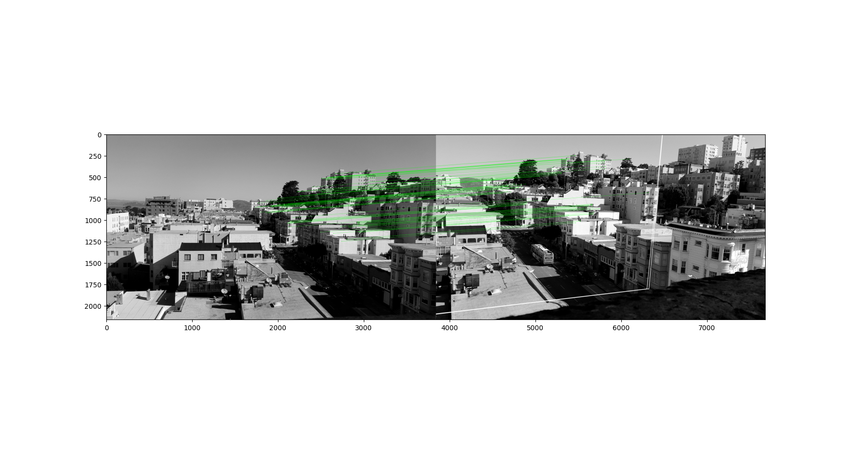
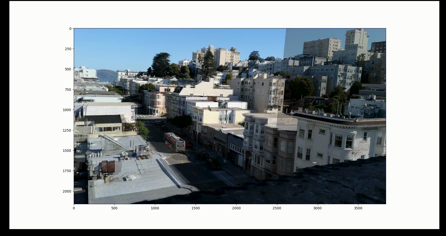
Our databricks notebook shows how Spark + FFmpeg can be used to optimize the bitrate ladder of a sample 4K video.
We can compute these statistics at the shot-level after segmenting our video with a udf like:
shots_schema = ArrayType(
StructType([
StructField("start", FloatType(), False),
StructField("end", FloatType(), False)
]))
@udf(returnType=shots_schema)
defshot_detection(uri, threshold=0.3):
"""
FFmpeg filters threshold sum of absolute differences
in video frames to perform shot detection.
"""
p = subprocess.Popen(
(
ffmpeg.input(uri)
.filter("select", "gte(scene,{})".format(threshold))
.filter("showinfo")
.output("-", format="null")
.compile()
),
stderr=subprocess.PIPE,
)
result = p.communicate()[1].decode("utf-8")
shots = [ln.split()[0] for ln in result.split("pts_time:")]
shots[0] ='0'
shots = np.array(shots, dtype=float).tolist()
shots = list(zip(shots[:-1], shots[1:]))
return shots if shots else [(0, -1)]
Next, our custom udf computes VMAF scores using FFmpeg. Spark helps to distribute our function over a grid of bitrates and resolutions to measure distortion with VMAF.
Using curve-fitting, we can determine the rate-distortion curves for various bitrate-resolution combinations.
@udf(returnType=T.ArrayType(T.FloatType()))
deffit_rd_curve(bitrates, vmafs):
bitrates, vmafs = np.array(bitrates), np.array(vmafs)
log_fit =lambda x, a, b, c: a * np.log(x + b) + c
popt, pcov = curve_fit(log_fit, bitrates, vmafs, maxfev=5000)
return list(map(float, popt))
Now, we can determine the shot-level optimal bitrate ladder by considering the pareto frontier for our computations.
But researchers made another observation: the point of greatest curvature in the rate-distortion curves for high-resolution encodings is often lying on the pareto frontier. Using this, researchers aim to regress this “knee-point” to further reduce computations.
In our model, we compute the second derivative of the rate-distortion curve to obtain the knee-point:
$$ \frac{d^2}{{dx}^2} \left( a * \log(x + b) + c\right) = \frac{-a}{(x + b)^2} $$
After computing these values for many video samples, researchers regress this distinguished value from content signals including spatial and motion features. In this way, informative content-based priors can be used to reduce the workload in optimizing the bitrate ladder for percieved quality.
The following udf, helps to extract image byte arrays for inference:
@udf(returnType=ArrayType(BinaryType()))
defvideo2images(uri, width, height,
sample_rate: int =1,
start: float =0.0,
end: float =-1.0,
n_channels: int =3):
"""
Uses FFmpeg filters to extract image byte arrays
and sampled & localized to a segment of video in time.
"""
video_data, _ = (
ffmpeg.input(uri, threads=1)
.output(
"pipe:",
format="rawvideo",
pix_fmt="rgb24",
ss=start,
t=end - start,
r=1/ sample_rate,
).run(capture_stdout=True))
img_size = height * width * n_channels
return [video_data[idx:idx + img_size] for idx in range(0, len(video_data), img_size)]
We can obtain image representations for our regressor using a ResNet pretrained on Imagenet.
model = ResNet50(include_top=False)
bc_model_weights = sc.broadcast(model.get_weights())
defmodel_fn():
model = ResNet50(weights=None, include_top=False)
model.set_weights(bc_model_weights.value)
return model
defpreprocess(content):
img = tf.io.decode_png(content, 3)
arr = tf.image.resize(img, [224,224], method='nearest')
return preprocess_input(arr)
deffeaturize_series(model, content_series):
input = np.stack(content_series.map(preprocess))
preds = model.predict(input)
output = [p.flatten() for p in preds]
return pd.Series(output)
@pandas_udf('array<float>', PandasUDFType.SCALAR_ITER)
deffeaturize_udf(content_series_iter):
model = model_fn()
for content_series in content_series_iter:
yield featurize_series(model, content_series)
We can use openCV’s implementation of optical flow to incorporate motion information. Furthermore, after determining the knee-point, Netflix researchers described sequential models to infer the remainder of the bitrate ladder.
If all this seems like overkill, you might prefer an AWS ABR service.
Stay tuned for more updates as we apply content-aware encoding techniques to improve visual quality subject to efficient streaming!
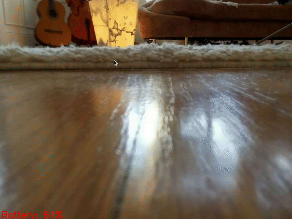
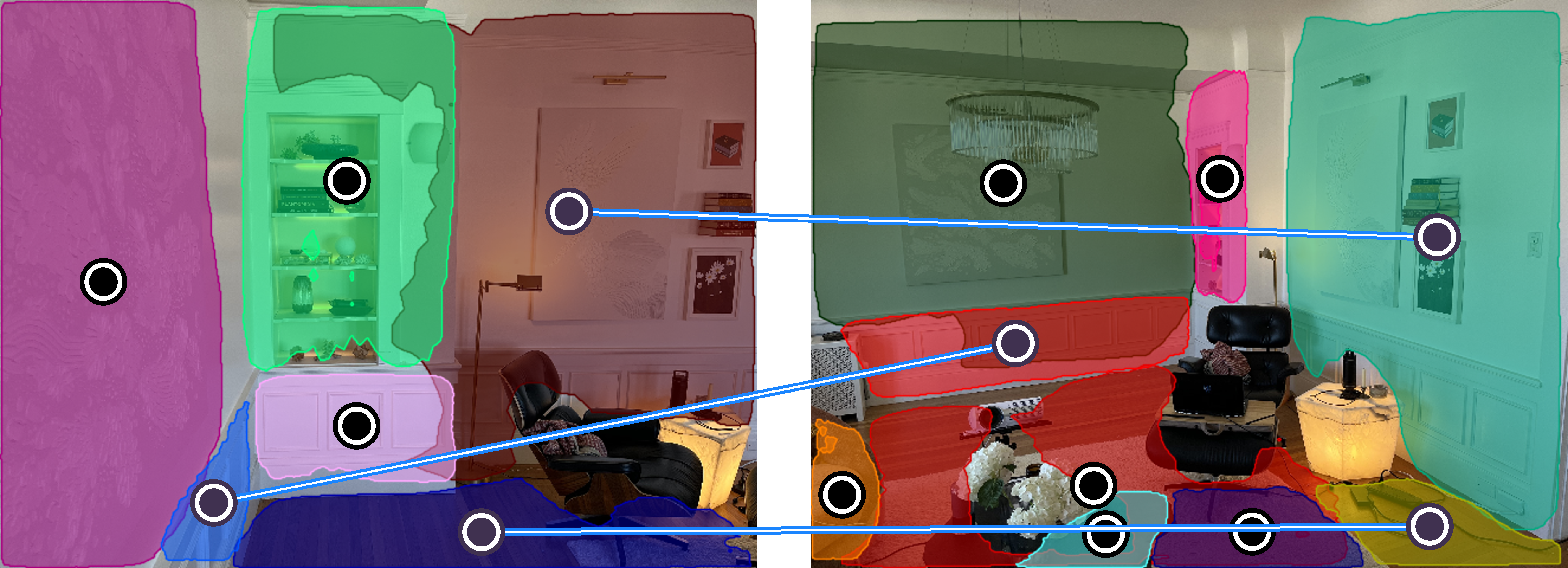
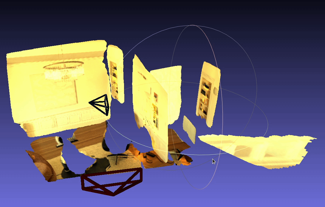
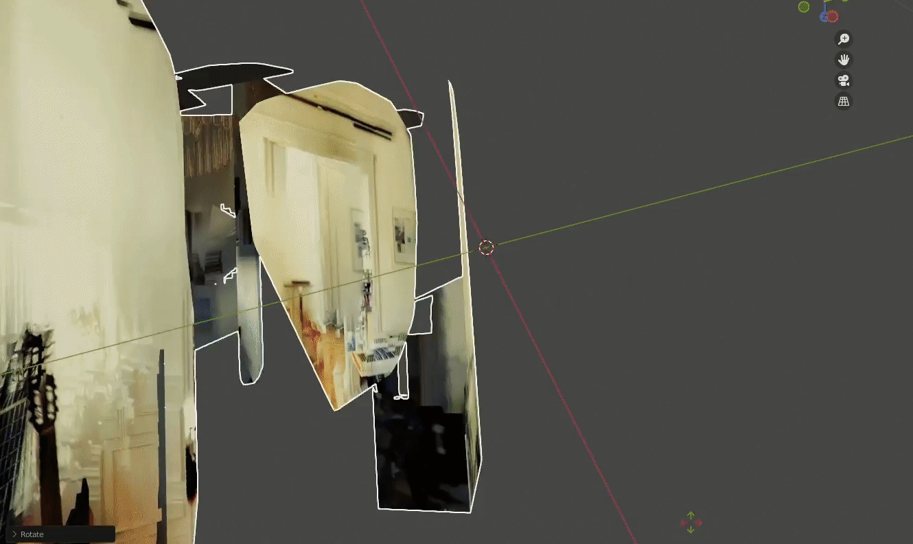
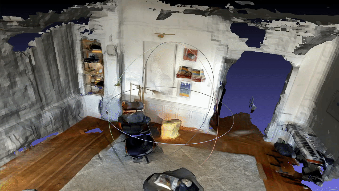
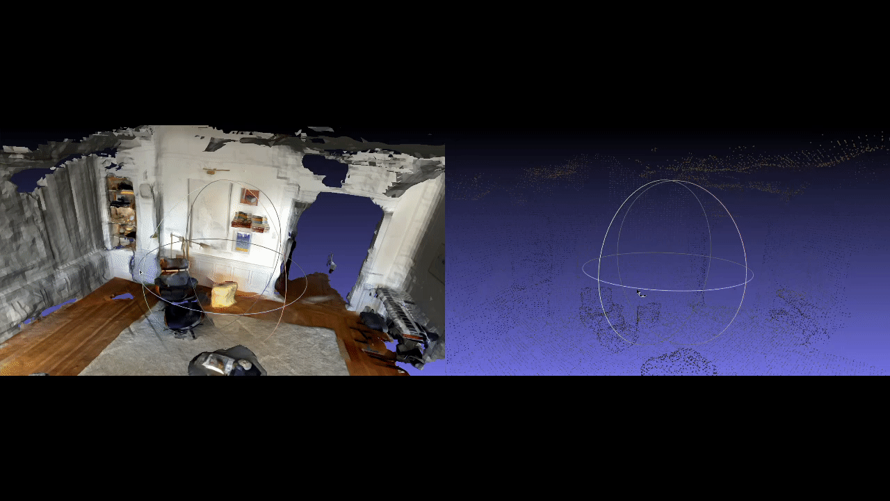
In recent experiments, we’ve generated high quality reconstructions of our apartment from video.
Learning the failure modes of these methods, you will move the camera smoothly, avoid bright lights, and focus on textured regions of the FOV.
If it all works out, you might spend more time recording video than processing it! Automating the data collection can really reduce the cost of mapping and reconstruction.
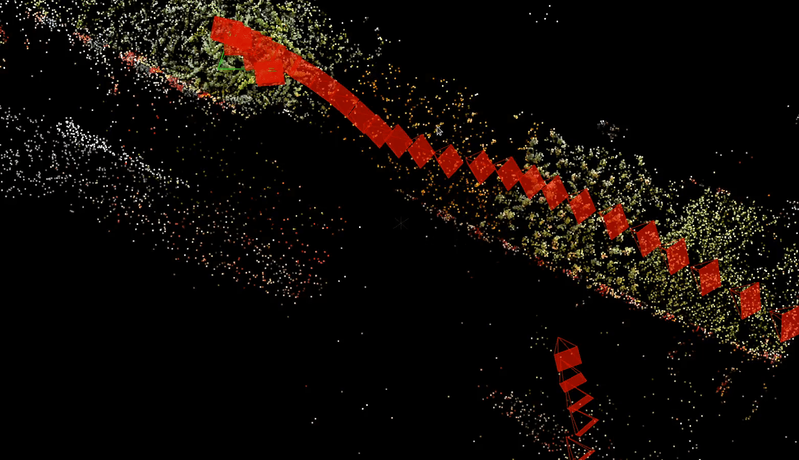
Compared to recording from a phone/tablet, drones move more smoothly and swiftly. At the same time, drones make it easier to set and vary the camera perspective.
The main limitation for drones might be battery life. To make the best use of the limited power resources, it is important to keep it moving while collecting data. But this frames another important challenge, obstacle avoidance and control.
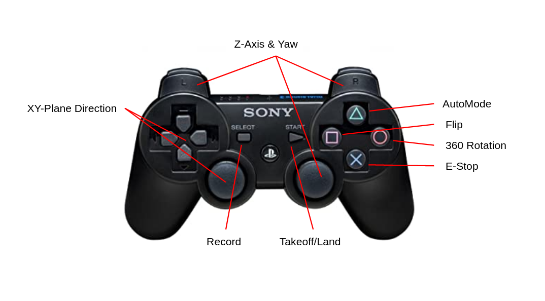
We find preconfigured maneuvers like flips and rotations will block the camera stream but in addition to images, we can stream IMU data and altitude to help estimate distance and scale.
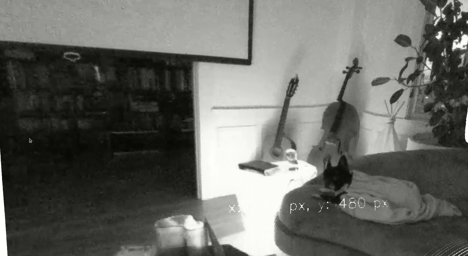
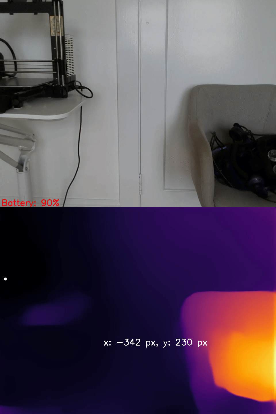
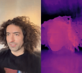
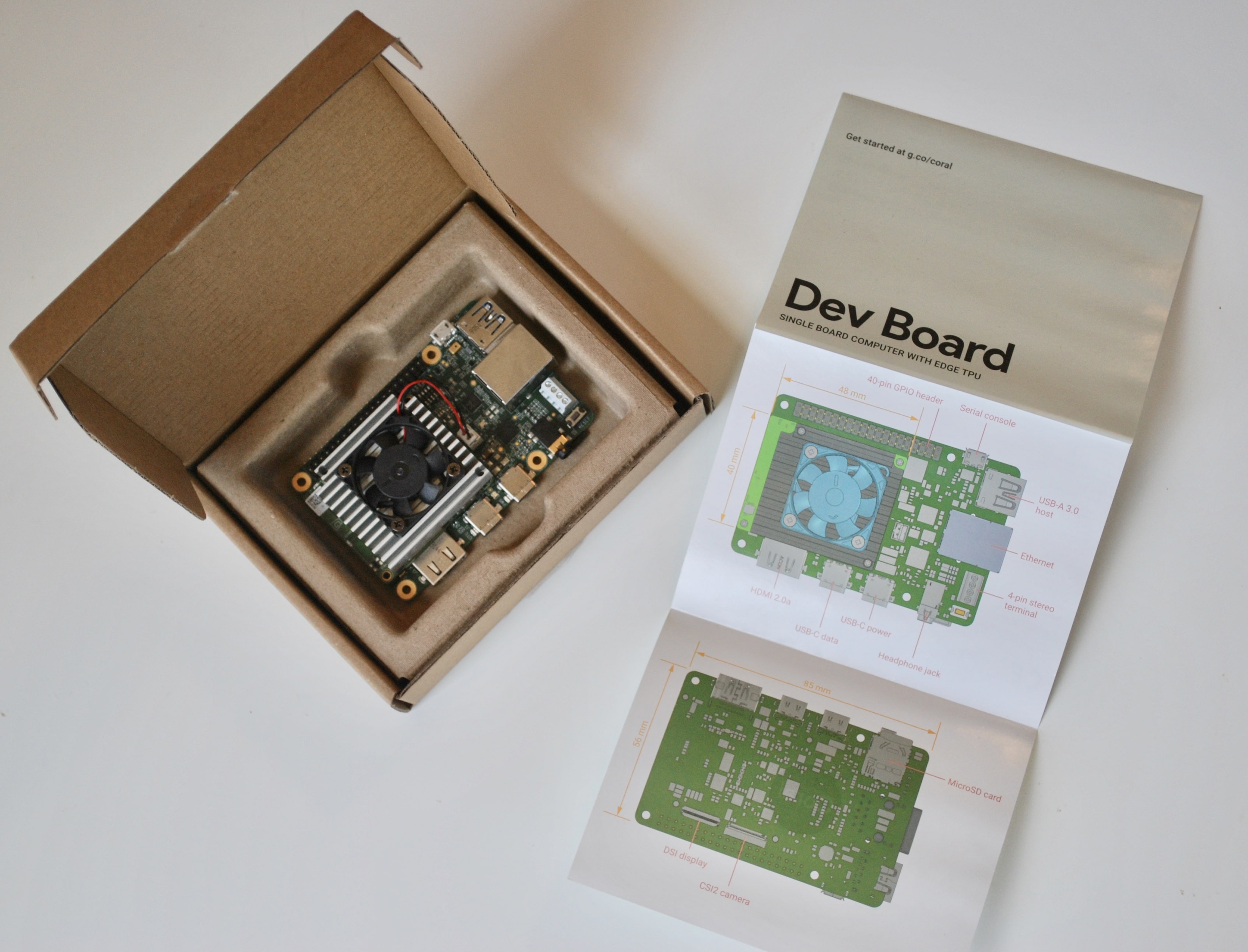
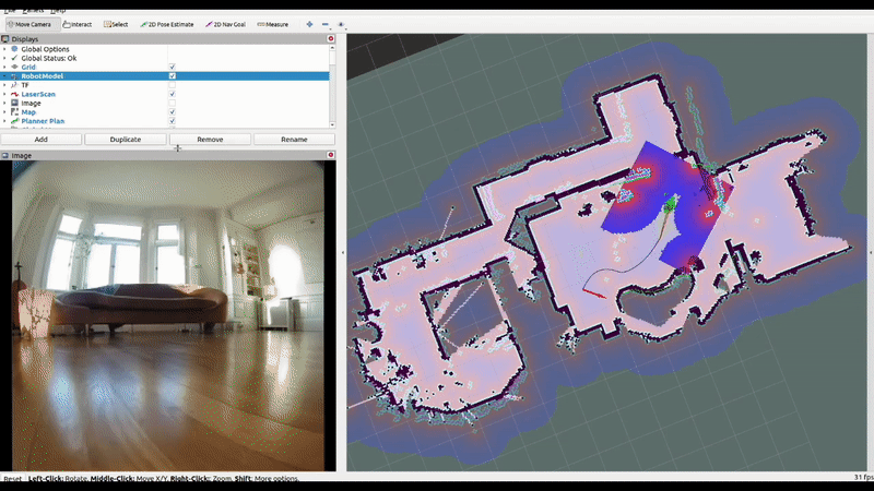
Now that our camera is flying, we wanted to avoid collisions so we incorporate depth estimation using MiDaS, which is accelerated by a USB Coral Dev stick.
We also added a detector to help select targets to track or follow, like we did with our turtlebot.
MiDaS for relative depth estimation tends to oversmooth at discontinuities and underestimate distance near the edges of the frame. There is impressive work to improve monocular depth estimation using boosting but this technique is not fast enough for our application.
Our drone’s perception could benefit from additional semantic and geometric constraints.
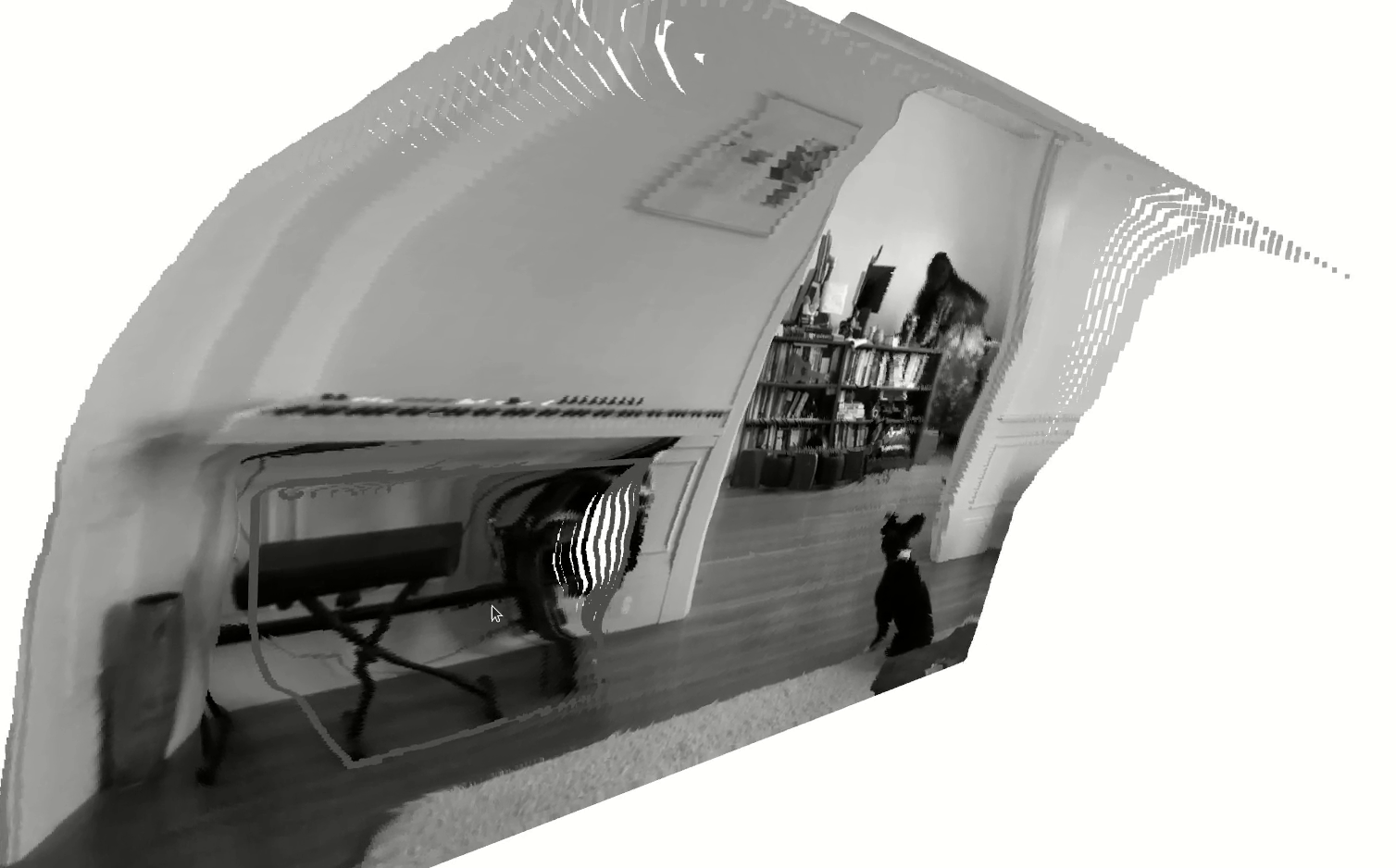
Apartment spaces typically feature open spaces with planar surfaces so we experimented with the sparsePlanes demo to get a sense for how plane-fitting might help.
With some reductions and hardware acceleration, it may be possible to run this model in real-time. Though both plane fitting and monocular depth estimation have shortcomings, they seem reliable in finding the deepest region of the image plane.
This inspires a navigation strategy: orient the camera toward the deepest part of the FOV. Assuming well-paced forward motion, this simple behavior can be effective in obstacle avoidance while fathoming an unmapped space.
Putting our drone’s yaw under PID control, we orient the drone toward the deepest part of the image plane. In this way, we can use the smoothness bias of MiDaS’s depth estimates to guide us toward safety with depth-first exploration.
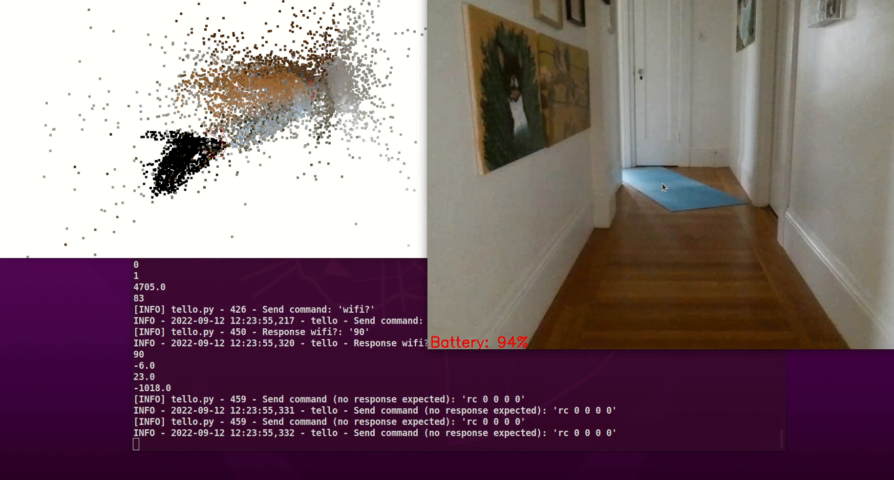
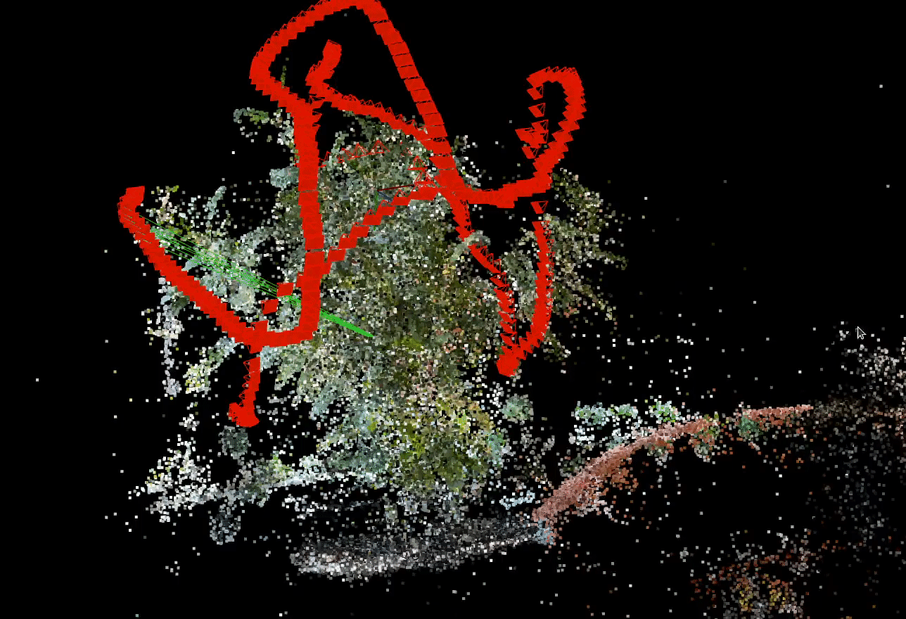
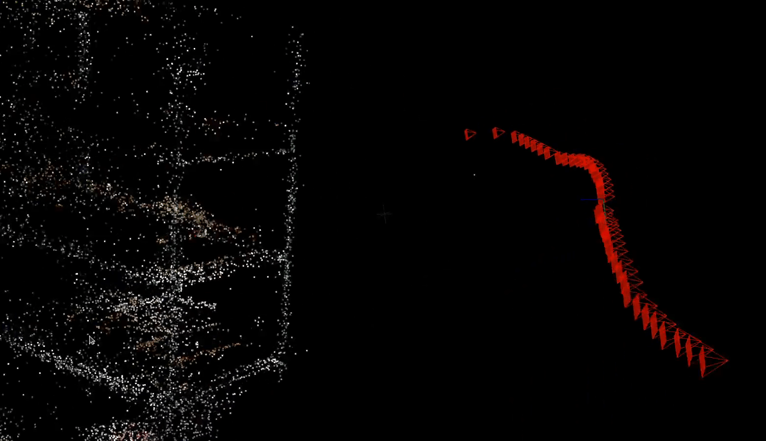
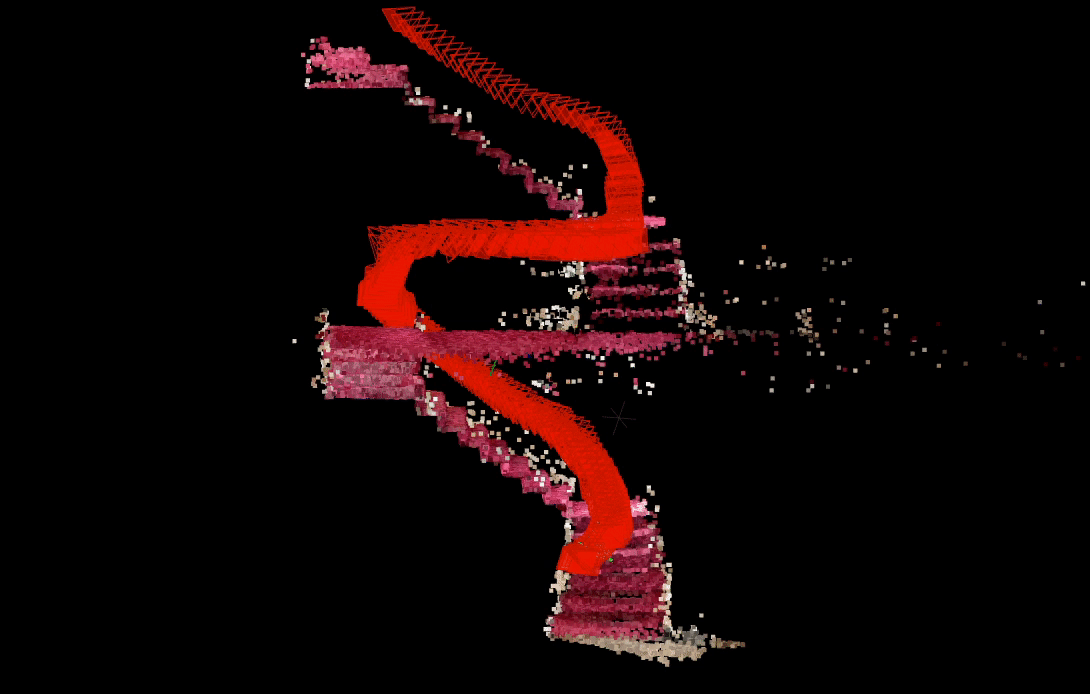
Since we want to make our drone capable of navigating unseen spaces, having the abililty to generate a map in real-time is important, so we experimented with DROID-SLAM.
We also evaluated an optimization-based monocular VSLAM method: PL-VINS. This lightweight method uses both point and line features with an implementation of line segment detection streamlined for the pose estimation use case.
With some of these fundamentals, we can help our drone quickly scan a space before the battery dies. We can monitor battery levels and develop an emergency landing behavior before it reaches 9%.
Using this platform, we can scale up to scanning larger spaces with a swarm!
With a low barrier for entry, the Tello drone made it easier to consider in-flight video capture for reconstruction. Automating the data collection process can both reduce the need for humans to carefully capture a space and increase the overall quality of the produced reconstruction.
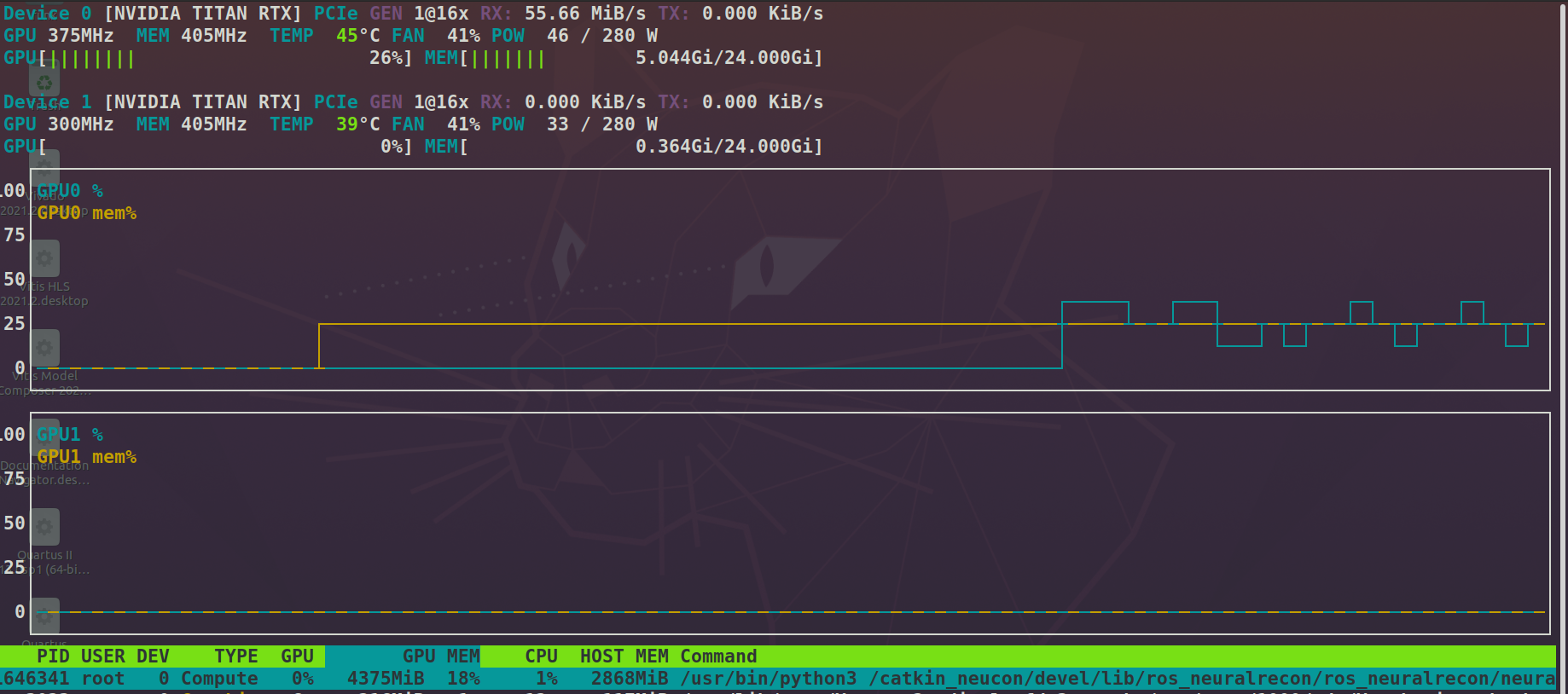
title: “Becoming CUDA Capable”
date: 2021-11-12T08:06:58-07:00
tags: [“GPU”]
ML on GPUs
Generally speaking, machine learning model training & inference is computationally expensive, so most practitioners know to try using GPU acceleration, if available.
Historically, these optimizations required expertise in GPU programming, especially using NVIDIA’s CUDA framework for parallel programming.
Recently, emergent best practices in model selection and transfer learning are abstracted into high-level apis, shifting the practitioner’s productivity bottlenecks from training models to getting data.
Assuming the upfront cost of developing a model to be amortized over the lifetime of it’s deployment, it becomes especially important to optimize runtime performance for your target hardware.
With NVIDIA’s latest TensorRT SDK release, one-line changes help you compile TorchScript or SavedModel artifacts optimized for fast inference using CUDA capable GPUs.
import torch
import torch_tensorrt as torchtrt
# SET trained model to evaluation mode
model = model.eval()
# COMPILE TRT module using Torch-TensorRT
trt_module = torchtrt.compile(model, inputs=[example_input]
enabled_precisions={torch.half})
# RUN optimized inference with Torch-TensorRT
trt_module(x)
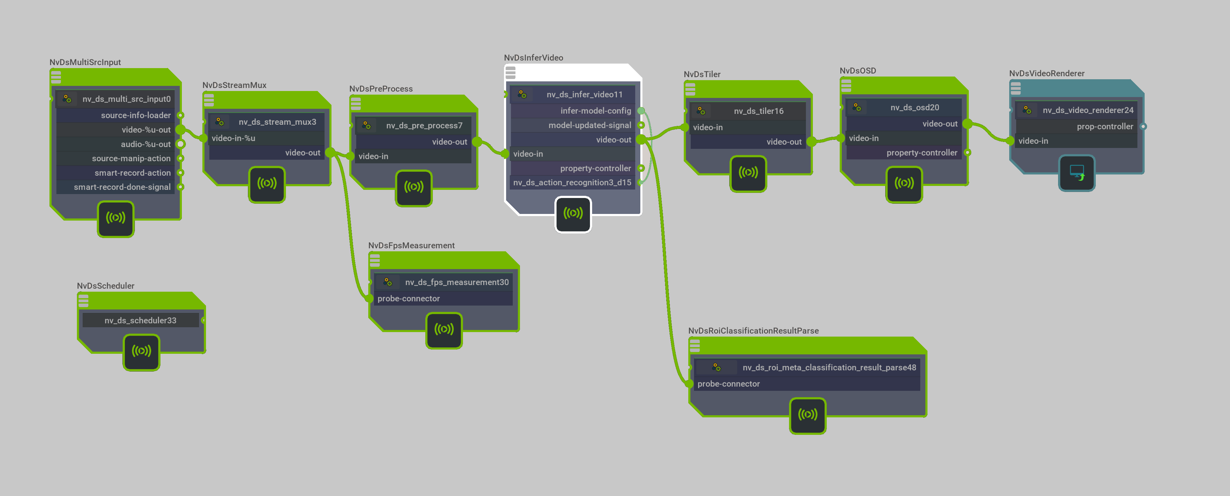
Likewise, building complex video analytics pipelines can be reduced to changing configurations, or even manipulating the Graph Composer GUI in the newest release of NVIDIA’s Deepstream SDK.
While it’s easier than ever to simply put our GPUs to work and enjoy increased productivity, we are even more bullish about learning the underlying technologies enabling these gains.
Though these MIT lecture slides compiled by Nicolas Pinto are 10 years old, they still offer an excellent motivation for GPU programming.
A key question is “How much will your workload benefit from GPU acceleration?” relating to considerations like “How parallelizable is your workload?”.
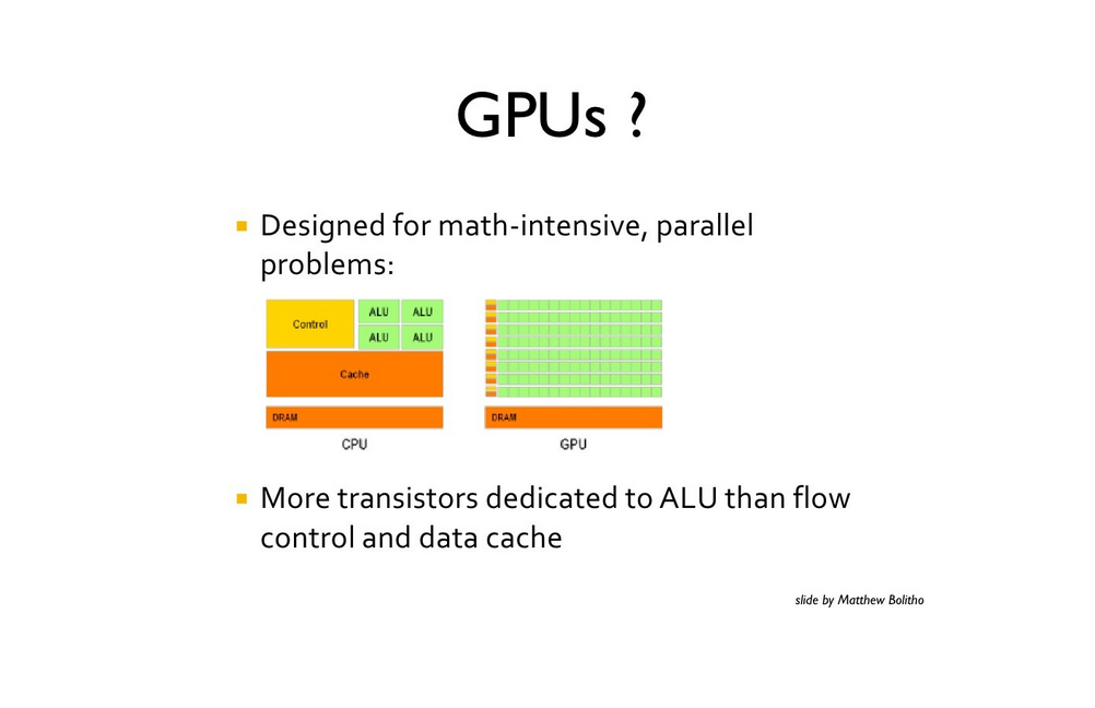
For many machine learning algorithms, training and inference entails repeated application of matrix multiplications, which can be parallelized through block multiplication. Appealing to Amdahl’s law we can estimate the theoretical gains expected through parallelized implementations.
The inherent data parallelism of certain ML workloads motivates a desire to apply more threads since CPUs are reaching physical limitations to achieving higher frequency.
Consider this excerpt from the slides referenced above:
ALUs are efficient at performing low-precision arithmetic operations, though less proficient in task parallelism and context switching. Thus compared to more general processing units, they use smaller cache and amoritize the cost of managing instructions streams through single instruction multiple data (SIMD) parallelism.
GPU Software
GPUs were originally intended to support computer graphics and image processing and traditional GPU programming required casting the work in terms of rendering passes over data represented as texture maps. Over time, support for more versatile programming models was introduced.
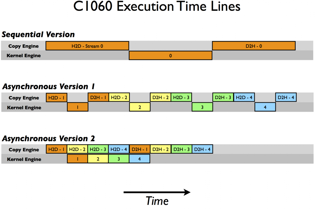
The CUDA API enables the practitioner to hide the latency of computations with GPU coprocessors by interleaving work asyncronously over CUDA streams.
Using the NVCC compiler and declaring suitable kernel functions, C programs can achieve dramatic performance improvements. These optimizations also depend on hardware specific attributes so autotuning the kernel to the device is an important part of efficient device utilization.
With all the compute capability of this hardware, memory bandwidth typically becomes the performance bottleneck. CUDA APIs support a rich memory hierarchy for caching and exploiting data locality. The CUDA library itself is also becoming optimized to reduce memory use, allowing for more/bigger models and training batches.
Learning More
Many of the library improvements are based on continued optimizations around the contraints of heterogeneous computing. And so even a rudimentary understanding of GPU programming & design can help the practitioner realize better hardware utilization and faster iteration. However, a deeper understanding frees the practitioner to advance the frontiers of GPU programming.
We are excited about developments in libraries like CUDA and hopefully this has primed you to learn more!
Consider these resources available by library or web:
In applied machine learning, engineers may spend considerable effort optimizing model performance with respect to metrics like accuracy on hold-out data. At times, more nuanced engineering decisions may weigh additional factors, such as latency or algorithmic simplicity.
Across many problem domains, approximate, algorithmic solutions are preferred to more accurate techniques with poor scalability. It’s said that “what’s past is prologue”, an idea which manifests in the most foundational of problem solving methods: use prior information.
At times, we want to discover novelty or anomaly by cross referencing new samples against historical instances. Doing so without paying a cost linear in compute or memory is where things get interesting.
In this post, we consider data sketching, which uses many algorithmic techniques common to ML to support approximate query processing (AQP).
What’s in a Sketch?
Data Sketching is concerned with the efficient analysis of massive and/or streaming datasets. For instance, how would you spot a port scan amidst a large volume of network traffic in real-time?
Due to the scale of the data, efficient often means sublinear complexity. For many modern challenges like streaming data, sketching offers the only known approach, so what is sketching?
To summarize, “data sketching” references a class of stochastic algorithms trading accuracy for speed, endowed with error bounds guaranteed by probablistic estimates. For a motivating example, consider the Bloom filter a basic archetype.
Bloom filters help to efficiently evaluate set membership over large datasets. Using multiple hashing functions, we can encode set membership into a binary array with a single pass over the data.
Later, we fingerprint a query with hash functions and lookup bits indexed in our array, taking the min to determine with certainty if we have never seen the element before. On the other hand, smaller sketches lead to hash collisions and so our parameter choices in this scheme directly influences the false positive rate.
This simple probablistic data structure powers efficient indexing of massive data while suggesting a template to consider similar queries. Simply by replacing bits with integers, we can increment counters to estimate frequency distribution with the CountMin sketch. More generally, sketching entails a dataset compression scheme tailored to answer certain queries.
At a high level, we:
initialize an approximation
observe data instances and increment our approximation
retrieve query results
Concerning our approximation, these techniques start by identifying an (hopefully unbiased) estimator for a quantity of interest. At times, methods use boosting with ensembles to reduce variance. Tail bounds like Markov’s or Chebyshev’s help to ensure control over error.
Another representative scheme, invented at Bell labs in the 70’s by Robert Morris, offers approximate counting. While an exact answer requires $$O(log n)$$ bits, we can reduce complexity by orders of magnitude with approximation.
Important entities in a datasets like popular or trending topics are simply frequent items (over some time range) so we can use sketches designed to identify the “heavy hitters”.
In large systems, performance can be dominated by tail effects prompting groups like Datadog to develop quantile sketches. Alternatively, KLL has better theoretical guarantees with an implemention in an Apache project.
Perhaps you are thinking we should simply sample our dataset. However, it isn’t too hard to find a failure mode for this approach. Consider the challenge of counting distinct elements in a multiset. Here, hyperloglog helps where sampling would fail for many practical instances.
Another industrial application concerns disaggregating ad impression counts by demographic factors. Far from limited to keeping counts, sketching techniques can also be applied to differential privacy!
Johnson-Lindenstrauss lemma helps us to sketch pairwise distance computations in large, high dimensional datasets. Dotting your data with random normal matrices, we can drop dimensions while maintaining an unbiased estimate of squared euclidean distance. Cauchy-Schwarz helps relate L2 norms to inner product so we can extend our sketch to approximate the dot product.
Locality Sensitive Hashing (LSH) is a related idea which helps us to quantize an embedding space, some use this to to scale & distribute distance computations after partitioning by bucket id. Sketching techniques like embedding and sampling can even be applied to compute matrix multiplications or traces.
Implicit trace estimation has applications in efficiently computing matrix norms and spectral densities with randomized numerical linear algebra. Even fundamental techniques like linear regression can be further reduced with subspace embeddings and streaming PCA can be realized as a “frequent directions” problem.
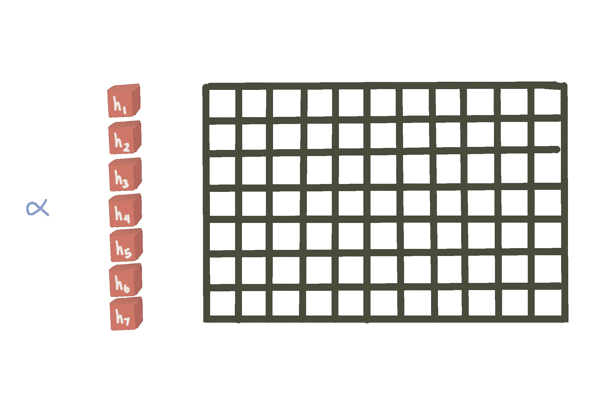
Streaming Eigenfaces
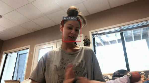
In the deepfake detection challenge, many contestants sampled or skipped frames from video to satisfy the contest’s performance constraint. Aiming to measure temporal inconsistency, we’ve explored different modeling strategies but have been unable to run inference on each frame. However, many faceswaps can appear intermittently as the quality of deepfakes varies.
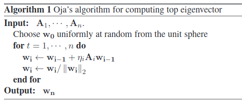
Using Oja’s method, we try applying streaming PCA for eigenfaces on tracked faces.
This model is much faster, parallelizable, and specialized to finding modes in face datasets. Understanding the modes, we look for large deviations betraying the faceswap.
We consider simple ideas to featurize top-K eigenvectors for a classifier or thresholding out-of-band reconstruction error in top-K eigenface projection. In the context of deepfake detection, we expect eigenbasis weights for faceswapped video to feature greater variance over time.
As the scale of training datasets increases, we are excited for fast, one-pass algorithms. Many complex video analytics workloads can be made more efficient by first extracting a cheap summary to reduce the effective search space & bandwidth. If these ideas interest you, check out how the research is trending here or here or here.
Advances in methods to generate photorealistic but synthetic images have prompted concerns about abusing the technology to spread misinformation.
In response, major tech companies like Facebook, Amazon, and Microsoft partnered to sponsor a contest hosted by Kaggle to mobilize machine learning talent to tackle the challenge.
With $1 million in prizes and nearly half a terabyte of samples to train on, this contest requires the development of models that can be deployed to combat deepfakes.
Although these deepfakes can involve faked audio, most deepfake samples involve a face swap. And so many contestants concentrate their efforts on developing face detection pipelines and applying deep learning to the classification task.
Having some recent experience working with motion transfer, we were eager to consider the complementary problem of detecting deepfakes.
After reviewing some of the data samples, our intuition was guided by the observation that temporal inconsistencies make deepfakes discernable during our review.
We want to exploit a weakness in the making of deepfakes. Specifically, these methods often don’t explicitly enforce a temporal smoothness constraint.
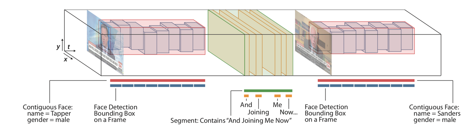
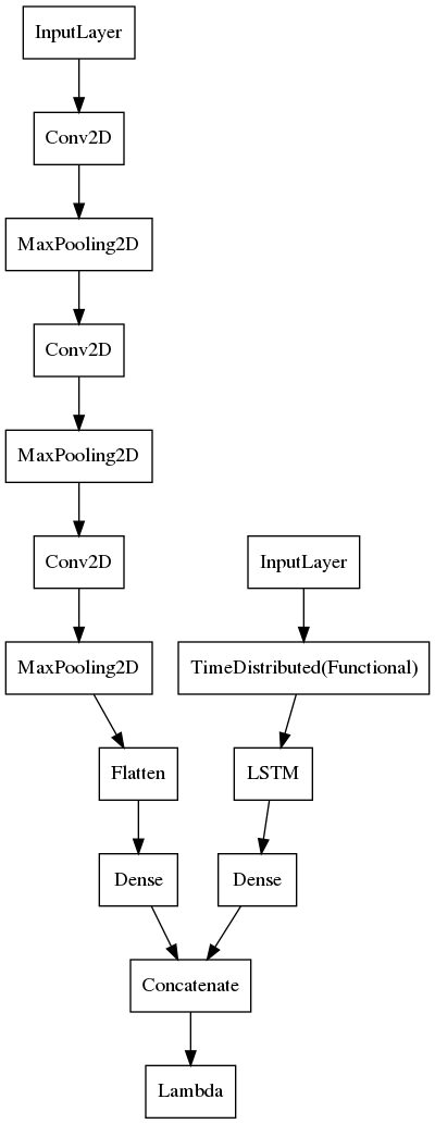
That is why we were especially interested in a video analytics pipeline which detects and tracks faces to construct feature descriptors over time for a sequential model.
The volume of the data requires some tricks to effectively process the data. In fact, the contest submission must finish analyzing 4000 videos in under 9 hours.
We released a kernel that shows how we can skip frames and apply object tracking to quickly preprocess the data.
By incorporating a face embedding feature extractor, we can construct a sequential feature to feed into an LSTM. This model is basically a Long-Term Recurrent Convolutional Network with a face embedding as a fixed feature extractor.
The model is small and fast so it could be deployed as a browser plugin to validate video on the fly. We found this method to be a simple approach to detecting the discrepancies in deepfake video. The model could be improved if it were trained on more varied videos.
title: “Deepfake Detection With NVIDIA TLT 3.0 and DeepStream SDK”
date: 2021-02-25T10:00:42-08:00
tags: [“GANs”, “GPU”, “computer vision”, “video”]
draft: false
Last year, over 2 thousand teams participated in Kaggle’s Deepfake detection video classification challenge. For this task, contestants were provided 470 GB of high resolution video and required to submit a notebook which predicts whether each sample video file has been deepfaked with a 9 hour run-time limit.
Since most deepfake technology performs a faceswap, contestants concentrated around face detection and analysis. Beginning with face detection, contestants could develop an image classifier using the provided labels.
Many open-source face detection libraries were considered over the contest. Aside from differences in deep learning framework, some implementations featured multi-task learning to offer facial keypoints or face embeddings in addition to bounding boxes. And because of the time-constraint, implementations supporting batch inference mode were important for faster performance.
Nonetheless, the volume of test data is too great for a frame-by-frame analysis so most contestants sampled the video a la bag-of-frames, aggregating inference results to the video level and disregarding time-space info.
Some participants used object tracking to associate bounding boxes over time for sequential models. However, fast and robust multi-object tracking is challenging enough to limit exploration during the contest.
NVIDIA’s DeepStream SDK shines in processing video with cascades of detectors and classifiers and integrates nicely with the new TLT 3.0 to train custom models.
In the remainder of this post, we highlight a simplified workflow in developing custom video classifiers using NVIDIA’s ecosystem.
For starters, this repo features reference deepstream sdk apps that you can deploy on a Jetson Nano or other compatible hardware.
We are interested in the detect-track-classify pattern using pre-trained face detection models. A similar demo performs face detection and tracking to redact personally identifiable info in video.
Bag-of-Frames Classifier Approach
Feature Engineering
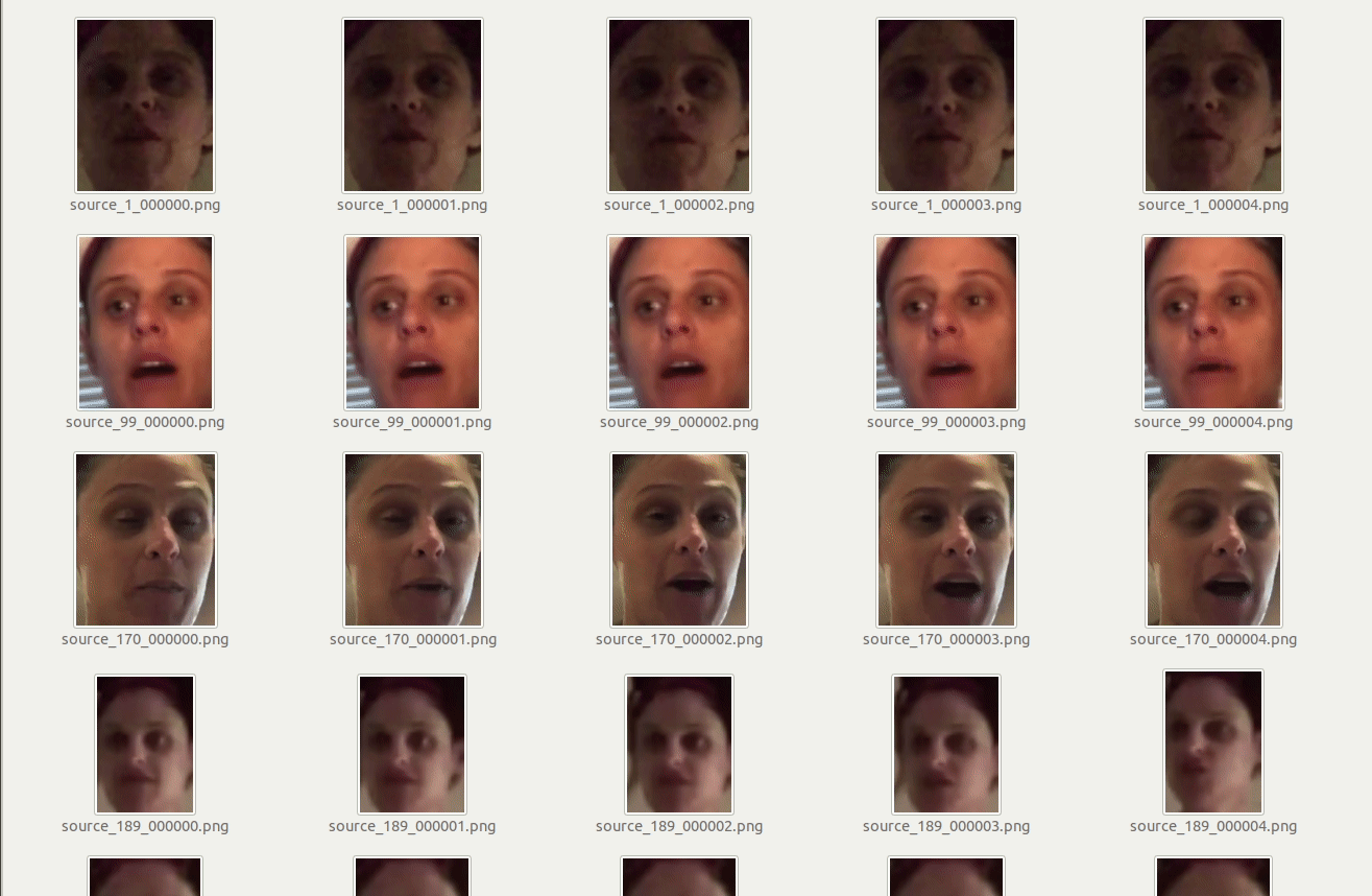
After pulling and launching this docker container, we update the deepstream config file to reference a face detector. Then we can extract bounding boxes of tracked faces from our directory of videos before writing results in KITTI format.
Note: The deepstream sdk 5.x has a memory leak with long video processing jobs due to a gstreamer issue. For now, we recommend using versions 4.x or patching versions 5.x for more stability.
Here, we note that some sample videos were filmed in portrait mode. To maintain an appropriate aspect ratio for the model, it is easiest to pad the video with ffmpeg after renaming files with a bash command.
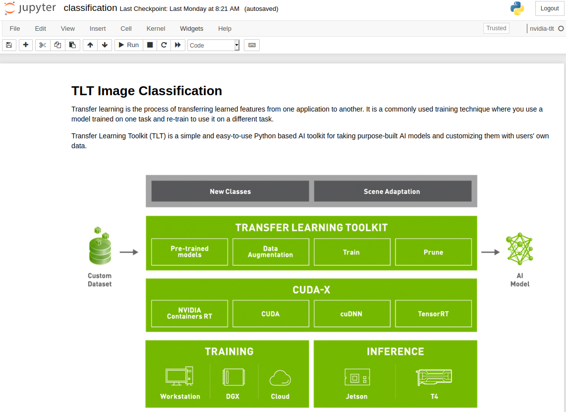
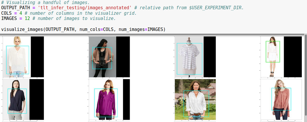
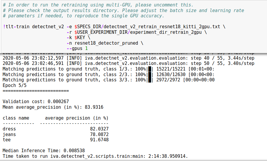
After indexing the locations of faces in time-space for our video corpus, we can extract images into a directory structure suitable for fine-tuning a ResNet base CNN for image classification with the new NVIDIA Transfer Learning Toolkit (TLT) 3.0.
Training a Deepfake Classifier with TLT 3.0
Using the TLT 3.0 requires minimal setup to fine-tune an optimized classification model on your dataset. After pip installing the launcher in your environment, you can download the Jupyter notebooks and training configs from the NGC Catalog. For this example, we use the notebook resources under the classification/ directory.
This notebook will:
Take a pretrained resnet18 model and finetune on our dataset generated earlier
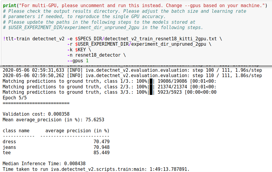
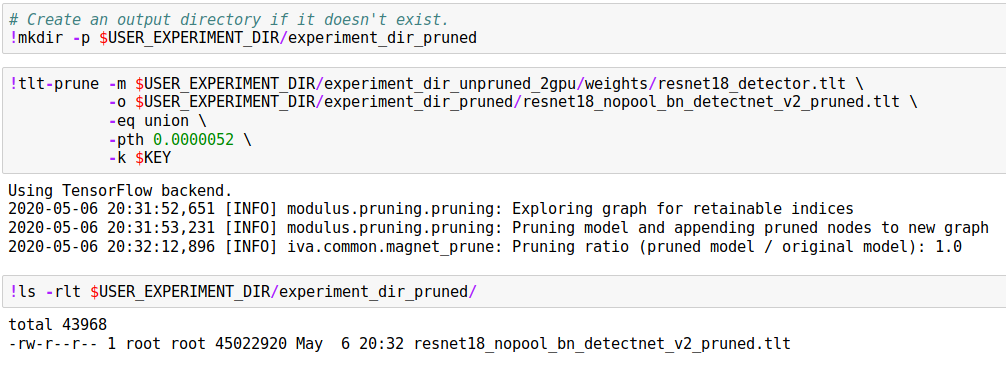
Prune the finetuned model
Retrain the pruned model to recover lost accuracy
Export the pruned model
Run Inference on the trained model
Export the pruned and retrained model to a .etlt file for deployment to DeepStream
You can modify the default training parameters to your liking by editing the classification_spec.cfg file located in the specs/ directory. In under an hour, we had a model ready to deploy with the DeepStream SDK.
Model Deployment
After fine-tuning our model, we add it as a secondary classifier in the face detection pipeline as described here to infer whether a face crop is likely a deepfaked.
So far, the DeepStream SDK has helped to quickly and robustly index face locations in our video corpus. Within the NVIDIA ecosystem, using TLT helped to quickly establish powerful baseline image classifiers via transfer learning.
Video Classifier Approach
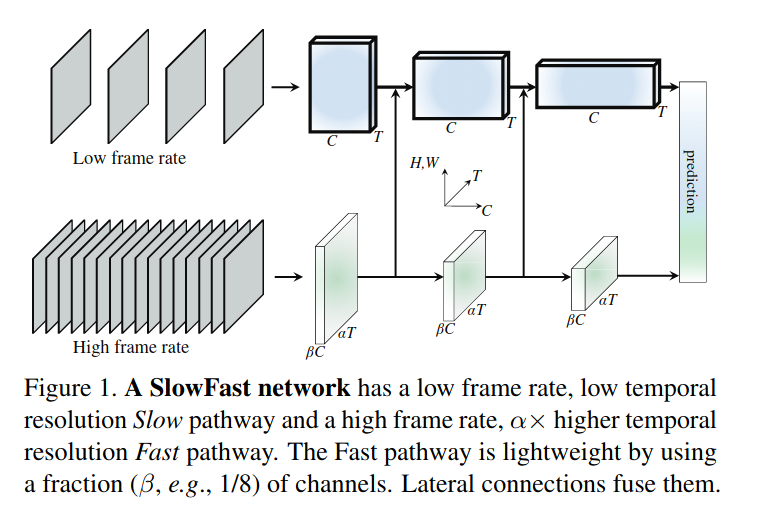
Next, we consider a video classifier used to achieve state-of-the-art results in human activity recognition, SlowFast.
The SlowFast researchers describe the biological inspiration behind the work, mimicking the function of P and M type retinal ganglion cells.
Stucturally, SlowFast uses two pathways sampling video at different rates. The slow pathway samples video frames at a lower frequency and is designed to capture high-level image features like color/texture. Conversely, the fast pathway samples video frames at higher time resolution but lower spatial resolution.
Feature Engineering
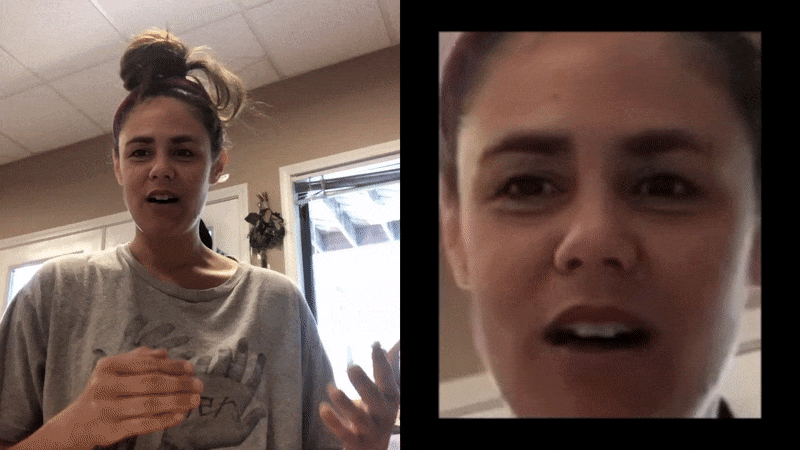
Since we have extracted thousands of videos cropped to the faces using the DeepStream SDK, we can assemble the face crops back into videos.
Then we label each clip to train our video classifier using the SlowFast model. We used a sample config that assumes a Kinetics Dataset formatted dataset.
We found the default learning rate too large for the model to effectively train on our dataset. Shrinking the learning rate by a factor of 10 resolved this for our dataset.
We also used transfer learning with a pretrained model for this new task.
The SlowFast model generates statistics like the top-k accuracy for an evaluation dataset and since we used a balanced training dataset with two classes, it was exciting to find 83% top-1 accuracy with minimal parameter tuning! We also believe additional accuracy gains can be made by refining our face detection pipeline to gather more training samples.
Summary
Winning contest entries reduced the video classification task to image classification through the bag-of-frames approach but there is plenty of additional information to use when we treat video sequentially.
Further work around the idiosyncrasies of the deepfake detection dataset, as well as hyperparameter tuning make video classifiers purposed to human activity recognition, attractive choices for this task.
We believe the SlowFast model is well-suited to the task of detecting faceswaps and in the sequel, we plan to cover some of these optimizations and compare to our LSTM model over sequences of face embeddings.
In our latest experiment with Depthai’s cameras, we consider visual localization.
This relates to the simultaneous localization and mapping (SLAM) problem that robots use to consistently localize in a known environment. However, instead of feature matching with algorithms like ORB, we can try to directly regress the pose of a known object.
This approach uses object detection, which is more robust to changes in illumination and perspective than classical techniques. And without the need to generate a textured map of a new environment, this technique can be quickly adapted to new scenes.
Localization from the Edge
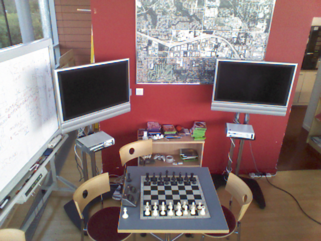
The researchers note that we can choose an object detector specialized for our scene. Since they demo the Chess scene from the 7-scenes dataset, our POC will use a detector which can identify objects like a television using depthai’s mobilenet-ssd.
The next stage of the pipeline includes models specialized to fit an ellipsoid to the object’s 3D bounding box for cheap & robust pose estimation. The authors regress parameters for approximating ellipsoids as the following example shows:
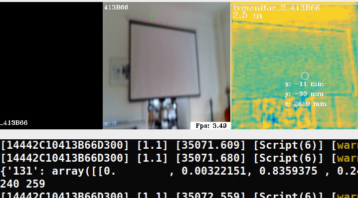
By converting these models into .blob, we can set up a NeuralNetwork node to run all the heavy inference at the edge.
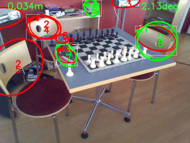
Here is a minimal example running the pipeline in an out-of-domain scene:
In the middle frame, we try overlaying ellipses, similar to the demo but clearly we need to retrain on our own data.
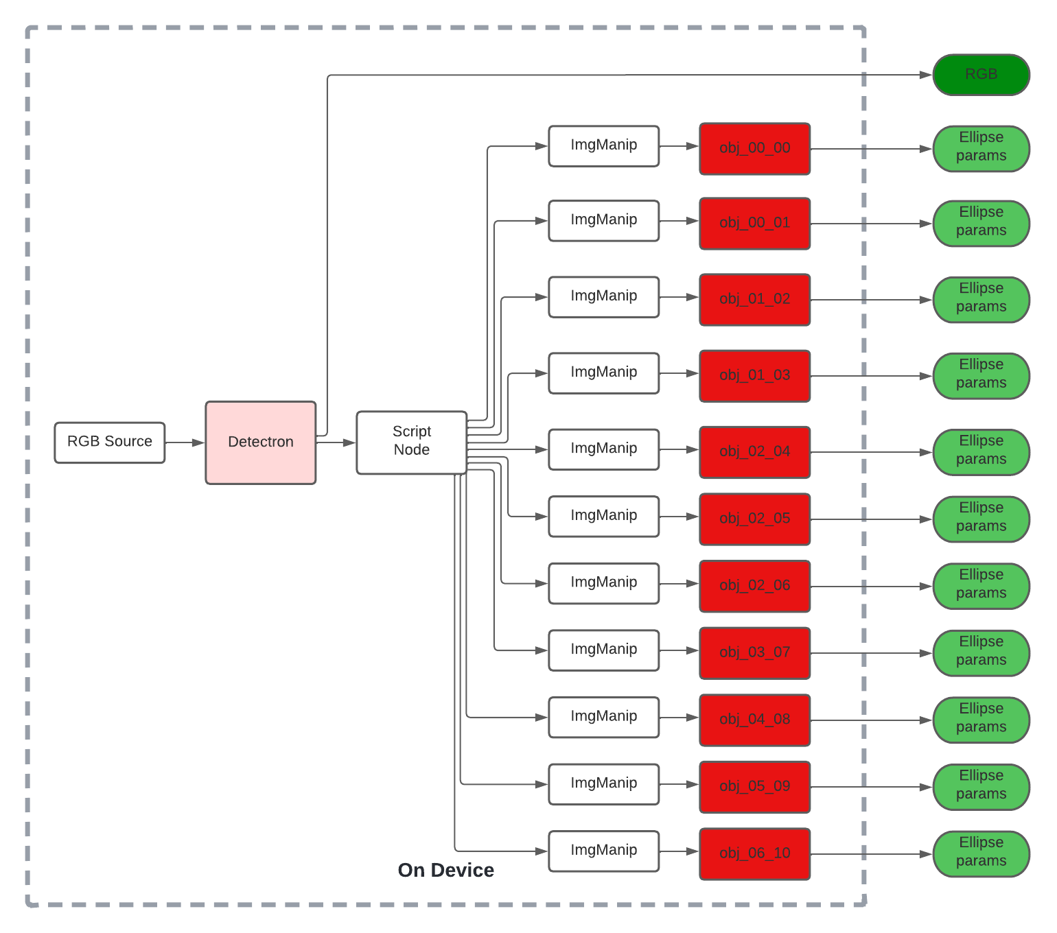
We could convert the remaining ellipsoid models from the research work into .blob format and use a script node to route messages to the appropriate NeuralNetwork node.
Such a pipeline with depthai’s SDK could look as follows:
The source can be a camera or even use the XLinkIn node to stream test samples to device.
We stream RGB frames from the camera to our object detection model, the authors used Detectron while our experiment uses mobilenet-SSD.
The inference results can be parsed with a script node to route each ImgFrame to the appropriate second-stage node for ellipsoid regression.
Finally, on the host device, we can incorporate this information into a RANSAC loop to produce the final camera pose estimate.
What’s Next?
We tried running a SOTA visual localization pipeline on device using depthai’s SDK after converting models to blob.
We can try training ellipsoid models at lower input resolution or using a lighter backbone than VGG-19 to speed things up.
We can even try integrating IMUData with the 9-axis sensor on camera.
Ultimately, we can annotate a new scene file for our setting and enjoy a robust localization method with much of the heavy lifting shifted to the edge.
And soon enough, we’ll run fast INT8 models on depthai’s new cameras which upgrade to Intel’s Gen 3 Movidius: Keem Bay, stay tuned!
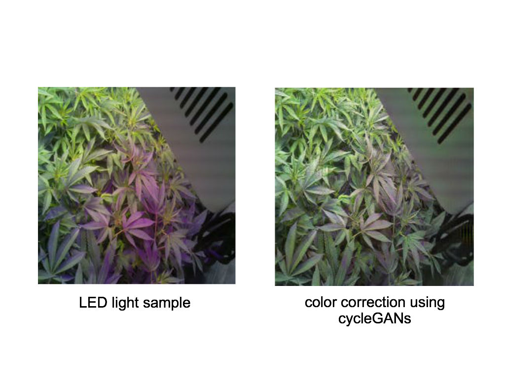
GANs represent the state of the art in image-to-image translation. However, it can be difficult to acquire aligned image pairs to learn the mapping between image domains. CycleGANs introduced the “cycle consistency” constraint to learn to transfigure images, transfer style, and enhance photos from unaligned source and target domain samples.
This technique has been used to render historic black & white images in full color or to represent an image in greater resolution but here, we explore applications in agriculture.
LED lighting used in modern greenhouses typically have more Blue and Red diodes since this is the part of the light spectrum that plants use for photosynthesis.
Besides making it more difficult for humans see, this unnatural lighting makes it more difficult to recognize yellowing which is one way plants show stress.
While there exists fancy shades for color correction, we adopt a computer vision approach for our environmental controller prototype.
Traditionally, color temperature correction requires some manual manipulation. Inspired by the impressive work around image superresolution, we applied this technology to learn a curve filter for color correction.
By curating an image corpus of greenhouse photos, both under unnatural color temperatures produced by LED/HPS lighting as well as images under a natural white light, we trained a cycleGAN to translate images from the domain of LED lighting to full-spectrum.
Compared to other applications, this example shows the ability of GANs to treat the image locally. We are excited to explore additional applications of this powerful new computer vision technique.
Convolutional Neural Networks have been a boon to the computer vision community. Deep learning from high-bandwidth image/video datasets can be computationally and statistically much more efficient using the inductive bias of strong locality. This streamlines inference over big datasets or on resource-limited hardware.
To model sequential dependence in short sequences of low-dimensional data, we have often used LSTMs. However, researchers have recently found success adapting Transformer architectures to learn from image and video, both applications traditionally dominated by CNNs.
Vaswani et al’s pioneering work in machine translation introduced the Transformer, which utilizes attention mechanisms rather than recurrent or convolutional layers while encoding sequential structure through sinusoidal positional embeddings. Transformers would pave the way for many advances in NLP, most notably influencing the design of BERT.
Image and video data decoded into arrays admit sequential/grid representations. Video is generally recorded at frame rates sufficient to spatially resolve objects of interest, implying some degree of local spatial smoothness in image and video.
The space-time locality of convolutional kernels helps us to efficiently exploit this regularity to learn models with low parameter counts. Furthermore, sharing kernel weights over sliding windows combined with pooling helps to impose translation equivariance, a symmetry we expect to observe for many labeled datasets.
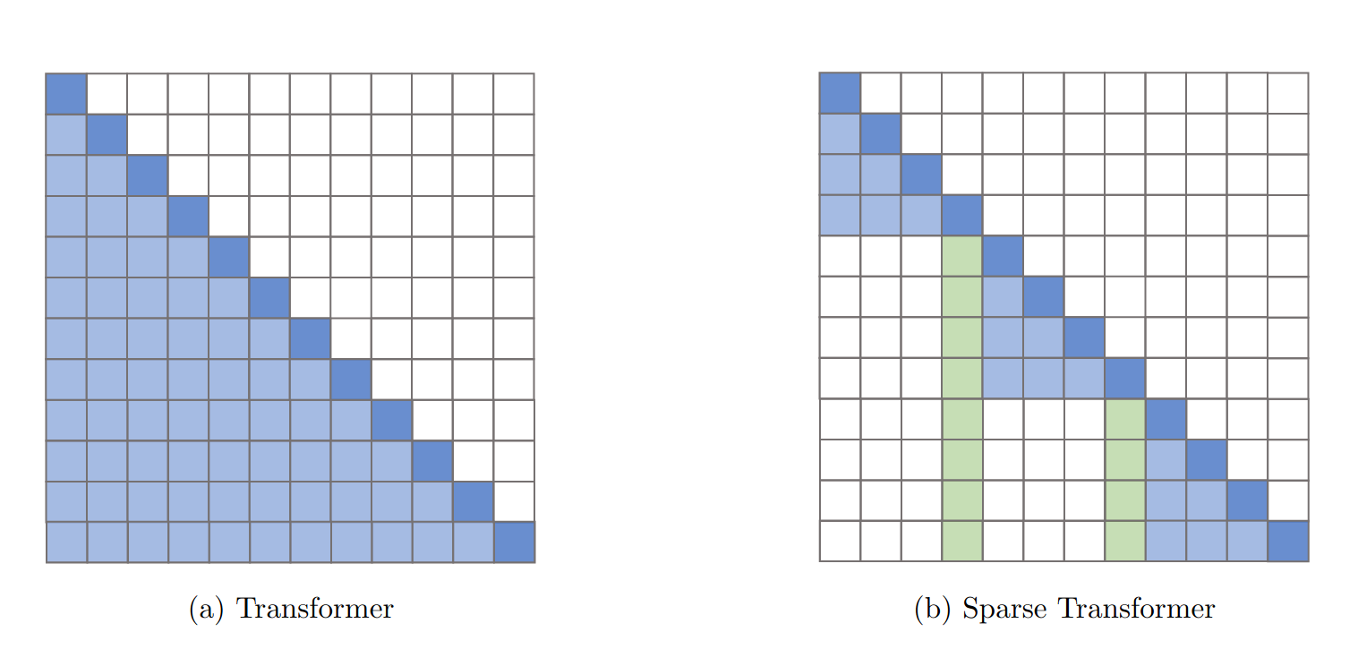
By comparison, self-attention in transformers is burdened by time & space complexity quadratic in the length of the input sequence. Despite this bottleneck, the model offers the capacity to learn from large-scale spatial interactions, spurring efforts to design more efficient transformers.
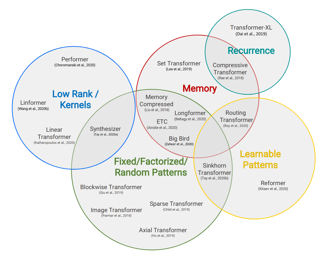
Google researchers describe a taxonomy of transformer variants, distinguished by the strategy used to sparsify attention.
Elementary reductions block or chunk the input sequences effectively quantizing the attention map. Similarly, strided or dilated attention helps to sample the input sequence. New schemes can be devised by combining these simple fixed patterns.
Advancing from handcrafted patterns, researchers considered learned attention maps. Some work reduces the token embedding space bucketing with LSH or using KMeans clustering.
Alex Graves suggests we consider “memory as attention through time” guiding research to introduce side-memory to limit the scope of a model’s attention.
Another conventient reduction is to assume a low-rank structure of the attention matrix to pass to a smaller N x k approximation (k « N). Ideas like kernel approximations and projection through Orthogonal Random Features offer this approach.
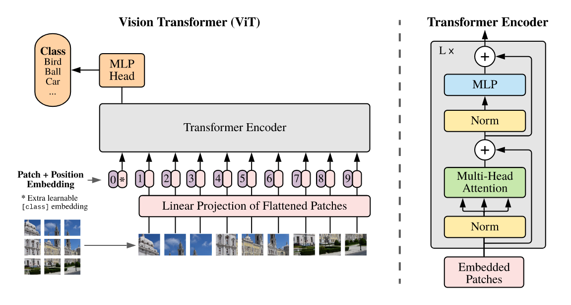
Vision Transformers (ViT) highlighted the potential for transformers in computer vision achieving SOTA performance comparable to models like Noisy Student and Big Transfer (BiT) across vision tasks after pretraining on larger (10M-100M) datasets.
The researchers reduced the compute bottleneck by tokenizing an image into patches while pointing out that specialized attention patterns suffer from a practical lack of hardware-accelerated implementations.
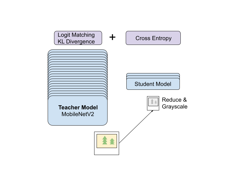
Transformers were further enhanced using Self-Supervised Learning (SSL) in Microsoft’s EsViT. Researchers borrow from BERT’s masked language modeling to incorporate local correlation information. This entails adding a term to the loss which encourages a student model to match a teacher’s soft label for a query patch, provided access only to distorted neighboring patches.
Facebook research into data-efficient Vision Transformers DeiT shows performant models trained on ImageNet-scale datasets. Researchers were interested in learning Transformer-based student models which benefit from the inductive bias of ConvNet-based teachers through knowledge distillation.
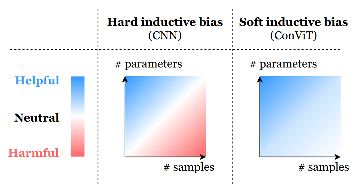
ConViT is another example hybridizing Transformers and ConvNets to endow the model with its inductive bias by initializing gated positional self-attention with convolutional priors using spatially-localized attention maps while relaxing any hard locality constraint.
The hard locality constraint enforced using convolutional layers helps mitigate the curse of dimensionality, but in the large data limit, may inhibit a model’s capacity to identify interactions occurring over larger spatial scales.
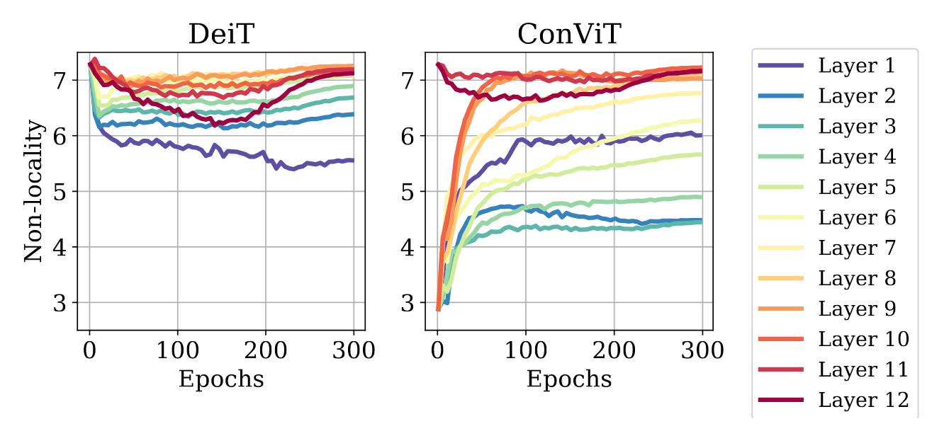
Comparing DeiT and ConViT with an aggregate metric of the attention-weighted distance between query and key patches, researchers find higher layers of ConViT attend to long-range interactions while promoting more diverse attention maps.
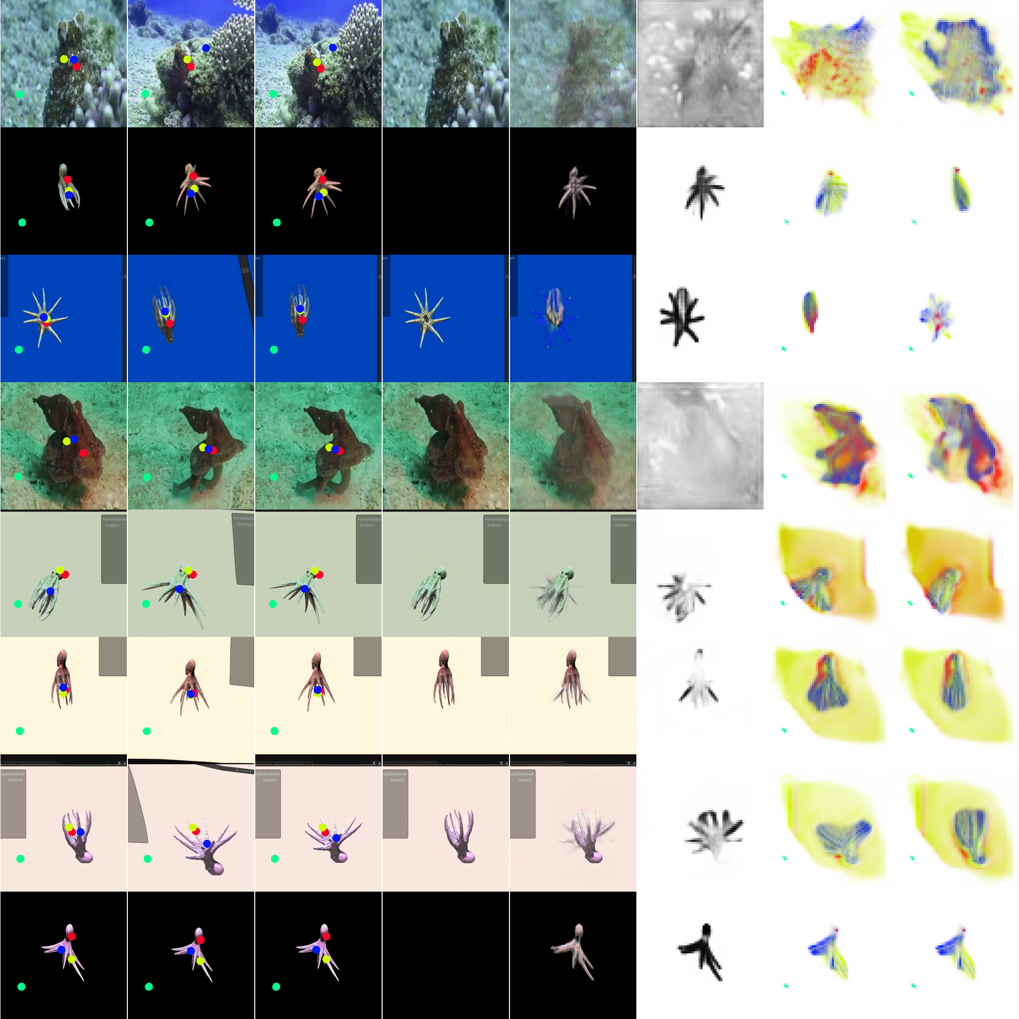
Considering the effect of initializing spatially-localized attention maps for training, we might ask whether attention maps concentrated in space-time could be useful in video object tracking. TrackFormer achieves tracking-by-attention after encoding frame level features extracted with a CNN backbone while dispensing with graph-based matching routines or appearance and motion models.
DeepMind’s Aloe applies self-supervised learning perform object tracking with transformers while characterizing the need to determine an appropriate level of resolution for input.
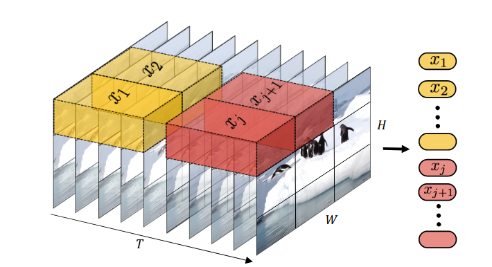
The Video Vision Transformer (ViViT) introduced a logical extension of spatial patches into the time dimension with tubelets:
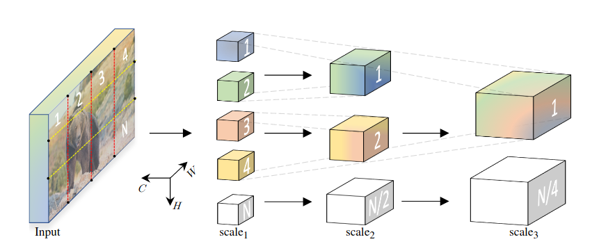
Multiscale Vision Transformers introduced a hierarchical pooling attention which researchers contend helps the model to break permutation invariance and make better use of temporal information.
Even as Transformer research trends toward stronger data-driven priors, FNet shows the power of structured mixing. Researchers note a nominal reduction in accuracy on the GLUE benchmark by simply swapping the $$O(N^2)$$ self-attention in a BERT architecture for the highly-optimized $$O(N *log(N))$$ FFT. Perhaps this work has an extension to the image domain by applying FFT over image patches.
FNet authors suggest applications as a student model in knowledge distillation for deployment on resource-constrained environments.
Stanford researchers were motivated to introduce similar reductions to reduce computational bottlenecks of 1x1 depth-wise separable convolutions in MobileNet.
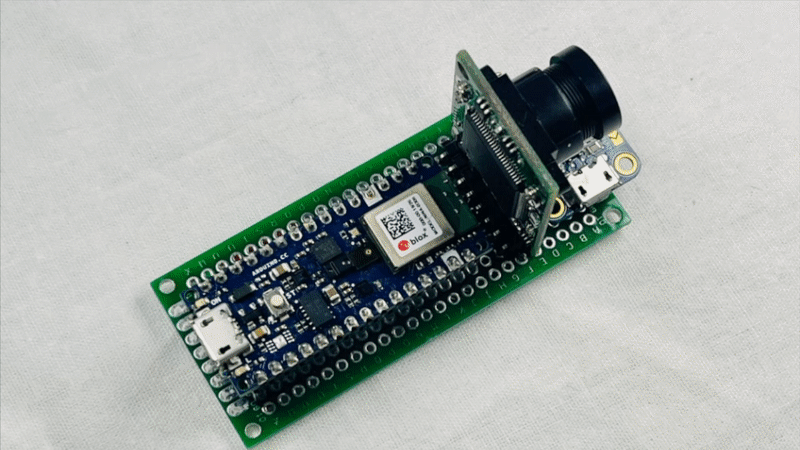
Others explored tiny Transformers for edge devices like the Arduino Nano BLE Sense, though limited by available tflite-micro ops. Making an addFNetMixercustom op for convolution by FFT could be an exciting contribution!
DeepMind researchers recently test the limits of Transformers over various data modalities including: audio, video, point cloud and text with Perceiver. This model utilizes cross-attention modules and latent factor projection to scale to high-dimensional input.
This success frames Transformers as the general purpose architecture and castes the utility of specialized architectures in doubt given the prevalence of big data. Indeed, researchers find Transformers generalizing well even to weakly-related tasks as training dataset scale increases.
After surveying the fontiers of research, we might conclude that specialized architectures like convolutional layers will remain en vogue for CV practitioners working in the small-medium data regime. But given sufficient volume of training data and/or aggressive augmentation and transfer learning, Transformers may reach higher performance using patterns learned over greater spatial scale.
We are learning to apply Transformers more generally and efficiently and expect to track increased adoption in ML systems.
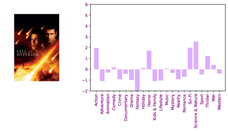
Our first vision experiment using Transformers trains deit_base_patch16_224 over 100K theatrical posters labeled with one of 22 primary genre labels. After a few ours of fine-tuning with 2 Titan RTXs, our classifier reaches 80% accuracy on the approximately balanced dataset.
Consider these sample images and corresponding model logits for qualitative review.
Encouraged by the classifier’s performance, we decided to apply transformers for image similarity to compare against previous work. Adapting the DeiT approach with a keras implemention, we pair a ViT-based student with a ResNet-based teacher using knowledge distillation to fine-tune a genre-classifier before fine-tuning with the triplet loss.
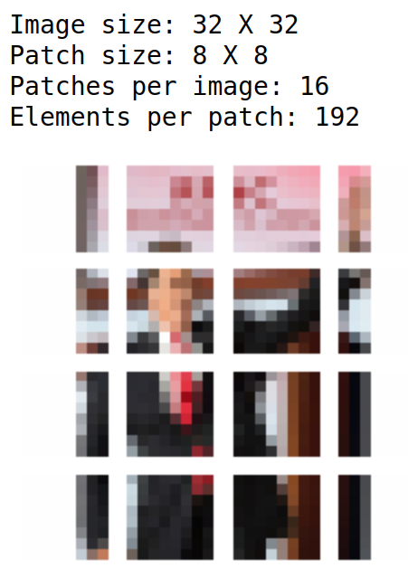
While the ResNet50 teacher takes 224x224 input, we consider much lower resolutions for the ViT student:
We conjecture this extreme reduction can be justified in observing that theatrical posters are quite structured by conventional motifs designed to signal theme & genre. Further, we anticipate simple patterns like color palette and featured objects convey most of the signal, whereas edges and text or otherwise high-frequency information may offer lower-order improvements, hindered somewhat by sparse representation.
This extensive ViT comparison indicates that transfer learning can be quite effective for training ViT models and augmentation helps to match performance of models pretrained on much larger datasets. They also find larger patch sizes perform better than smaller model architectures.
A recent paper offers tips for successful knowledge distillation which guided our augmentation strategy. Starting with a genre classifier trained from scratch with logloss, we fine-tune with triplet-loss.
As recommended in the ViT comparison above, we can use transfer learning, selecting similarity model architectures by evaluating validation accuracy in the upstream classification task, which is much faster to train!
With an average of two genres labels per title, our dataset lends to multiple representations and augmentation strategies. For instance, we might consider each genre label to provide a new training sample. On the other hand, by framing a multi-label classification, we aim to utilize covariance in genre label distribution to enhance our distillation.
In another experiment, we apply the Multiscale Vision Transformer (MViT) to videos cropped down to faces for deepfake detection. With small changes to the config MVIT_B_16x4_CONV.yaml, we reach 75% validation accuracy on the balanced binary classification task, training the model on roughly 7K samples from scratch.
We also tried training this model on more of the raw deepfake detection challenge videos. However, focusing the model on faces with a detection pipeline proved to powerful an inductive bias to pass up for this small sample.
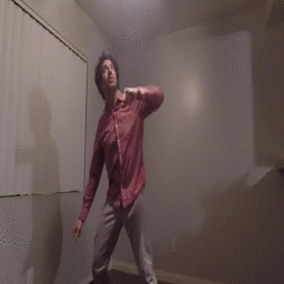
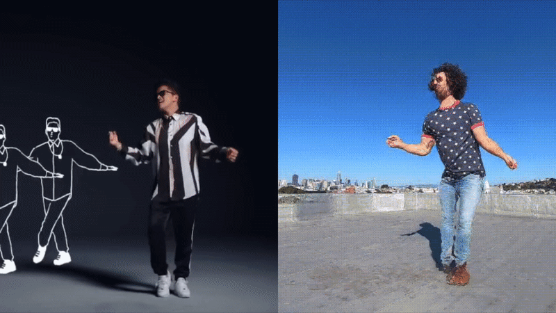
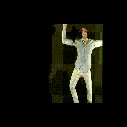
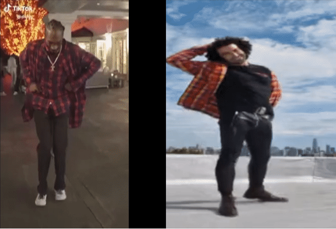
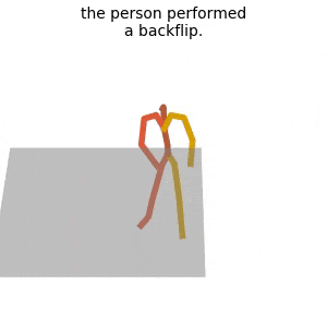
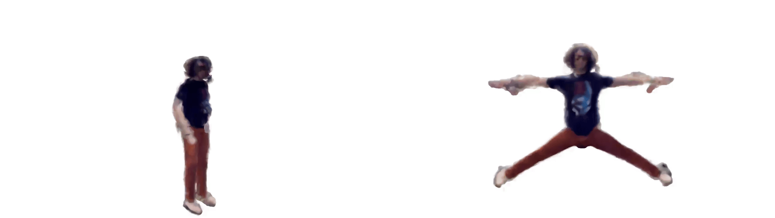
“Everybody Dance Now” offers a sensational demonstration in combining image-to-image translation with pose estimation to produce photo-realistic ‘do-as-i-do’ motion transfer.
Researchers used roughly 20 mins of video shot at 120 fps of a subject moving through a normal range of body motion.
It is also important for source and target videos to be taken from similar perspectives. Generally, this is a fixed camera angle at a third person perspective with the subject’s body occupying most of the image.
Producing this content is challenging because it:
Requires the user to move around in front of a camera for 20 mins
Involves training custom GAN from scratch
We want to explore model and implementation reductions with the goal of quickly producing ‘reasonable quality’ motion transfer examples in a live demo.
Before framing this further, let’s pause to consider specific challenges to producing qualitatively satisfactory examples.
Gallery of GANs Gone Wrong
In each of the following experiments, we use no more than 3 minutes of sample target video shot at 30 fps.
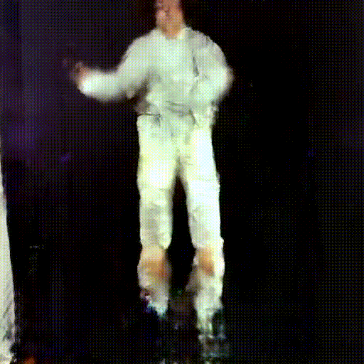
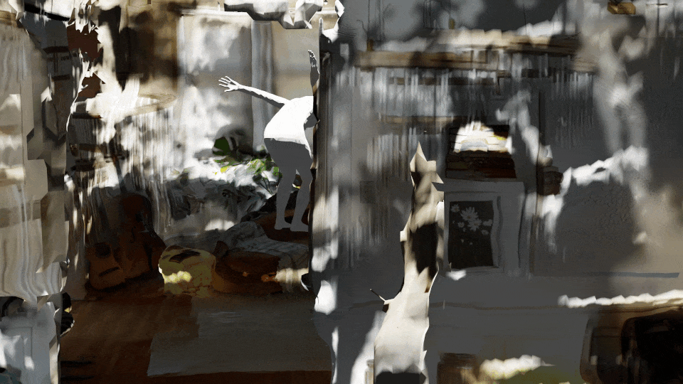
The first example shows how errors in pose estimation, particularly false positives on shadows, can be rendered as an unrealistic backup dancer.
Next, GANs are difficult to train, this example appears to suffer from mode collapse as well as challenges related to perspective from a tight framing.
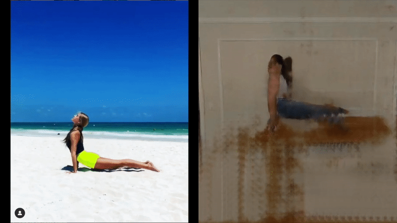
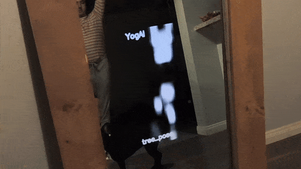
Pose estimation models simply don’t perform well in some body positions. Specifically, occlusion of the head or a relatively low framing of the upper body can impact pose estimate quality. The next example demonstrates an attempt at motion transfer of a yoga flow.
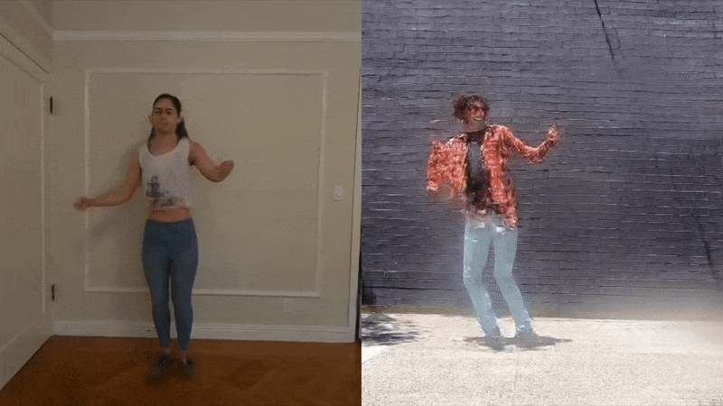
The next two are more convincing but each highlights the challenges in reproducing complex scenes.
Finally, we reach something closer to an entertaining example of motion transfer content.
Motivated by a sense of how our our experimental designs have impacted the quality of the renditions, we can constrain our demo to more consistently produce high quality examples.
Setting the Scene
Simple scenes are easiest to generate. This reduction will help us spend our practical compute budget refining models to produce hi fidelity renditions of the subject dancer.
Also, researchers emphasized slim fit clothing to limit the challenges of producing complex textures. For our purposes, we assume participants will wear attire typical to a tech or business conference.
Additionally, we want to assume the scene is an adequately lit booth with the space to frame a shot from a similar perspective to that of the source reference video.
The example above shows an idealized setting for our booth after training an image-to-image translation model on roughly 5 thousand 640x480 images.
Note the glitchy frames due to poor pose estimation at the feature extraction step on the source dance video.
Estimating Pose at the Edge
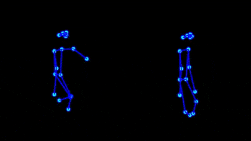
Motion transfer involves a costly feature extraction step of running pose estimates over source and target videos.
However, reference source videos should be assumed to be available and processed ahead of performing the transfer.
The new Coral Dev board (EdgeTPU) can run pose estimation at roughly 35 fps for 481x353 images using TFLite. For 640x480 images, we can run inference inline with frame acquisition at roughly 25 fps.
To achieve the greatest time resolution using hi-speed cameras, we would not block frame acquisition with inference and streaming, but could instead write images to an mp4. Then the video file can be queued for asynchronous processing and streaming.
Assuming a realistic time budget from a user in our booth, say 15 seconds, we can increase the number of edgeTPUs & hi-speed USB cameras until we can ensure acquiring sufficiently many training samples for the GANs.
We’ve also seen how pose estimate quality impacts the final result. We choose larger, more accurate models and apply simple heuristics to exploit continuity of motion.
More concretely, we impute missing keypoints and apply time smoothing to pose estimates en-queued into a circular buffer. This is especially sensible when performing hi-speed frame acquisition.
The main impact to final quality comes from poor pose estimates generated from the source video. As valuable reference videos processed ahead of time, these should be corrected manually if necessary.
Streaming the inference results to the cloud, we generate a training corpus for our image-to-image translation models.
Then the main bottleneck to quickly producing one of these examples in in training the GANs.
This reference implementation was run for roughly 8 hours on a GTX 1080 GPU. We want to get training times down to 1-hour so we will need something quite different.
Next, we discuss some implementation choices to expedite the production of motion transfer examples in a live demo setting.
Yo Dawg, I heard you like to Transfer…
…So we’re gonna apply transfer learning to this motion transfer task.
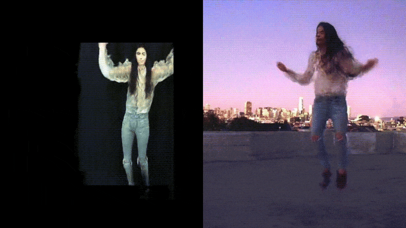
In other words, having trained a motion transfer model for one target dancer, we can use this model as a warm starting point to fine tune models for other dancers in the same scene.
Our setup thus far takes a few seconds to acquire images before running inference at the edge and pushing the results to the cloud. This means we have one hour to fine tune a model restored from a checkpointed one trained over hours ahead of time on our demo setting from above.
Since we use identical but flawed pose estimates from before, the following examples shows the same ‘glitch’ behavior. This is easily corrected in source video ahead of the demo day.
The above examples used transfer learning from checkpoints already trained to produce reasonable motion transfer renditions in our demo and rooftop environments, respectively. The booth setting on the left trained in only one hour, however, the complex rendition on the right took considerably longer.
This means we can invite users into our booth and let them move through a full range of motion in front of our array of cameras and edgeTPUs for a few seconds.
This setup will be acquiring thousands of photos and running inference in real-time before streaming results to the cloud.
In the cloud, we run a server to train the GAN for our one hour time budget before sending a user video links to hosted renditions.
By implementing pix2pix for cloud TPUs, we might expect similar results to be attainable in minutes!
Twisting the Task
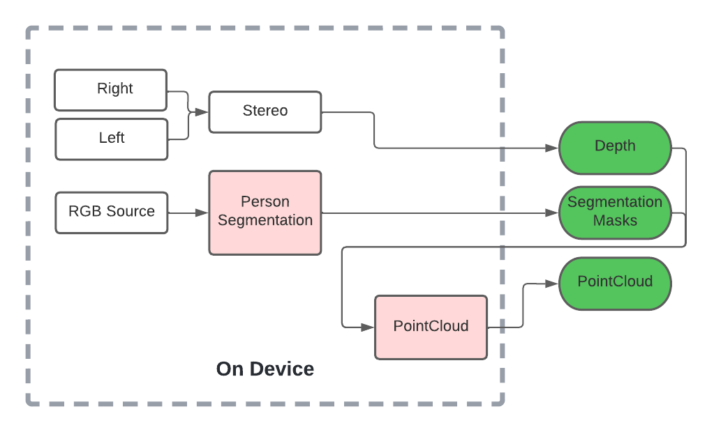
The person segmentation result, BodyPix, was published after “Everybody Dance Now” but offers an alternative to pose estimation for the intermediary representation used in motion transfer.
We might expect the BodyPix alternative to provide:
a smoother representation of body part location by virtue of representation as a region rather than a point
2D regions offer more implicit information on orientation than can be encoded with a line segment
greater pose resolution with 24 regions compared to 19 keypoints w/ pose estimation
The model is only available as a demo to use with tensorflow.js in the browser. For our proof-of-concept, we modify the demo so we can build the dataset to leverage person segmentation for motion transfer.
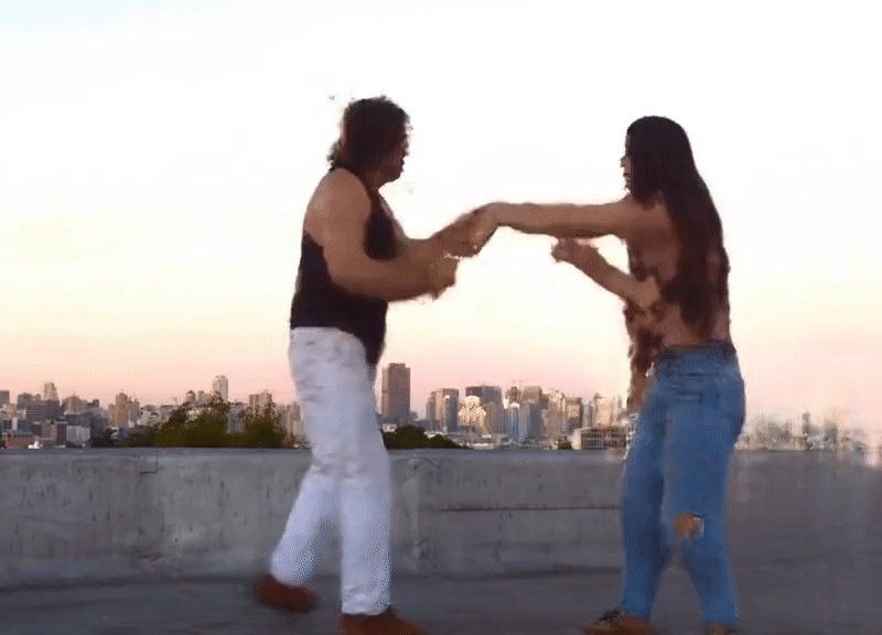
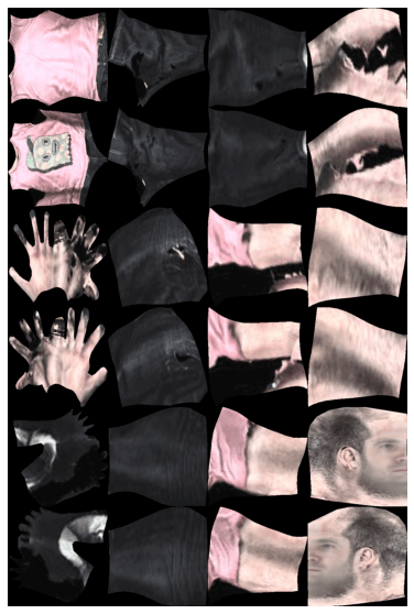
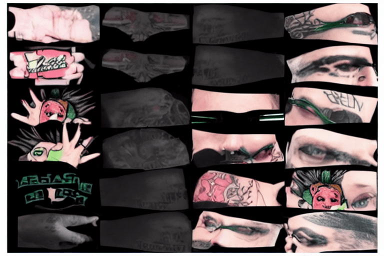
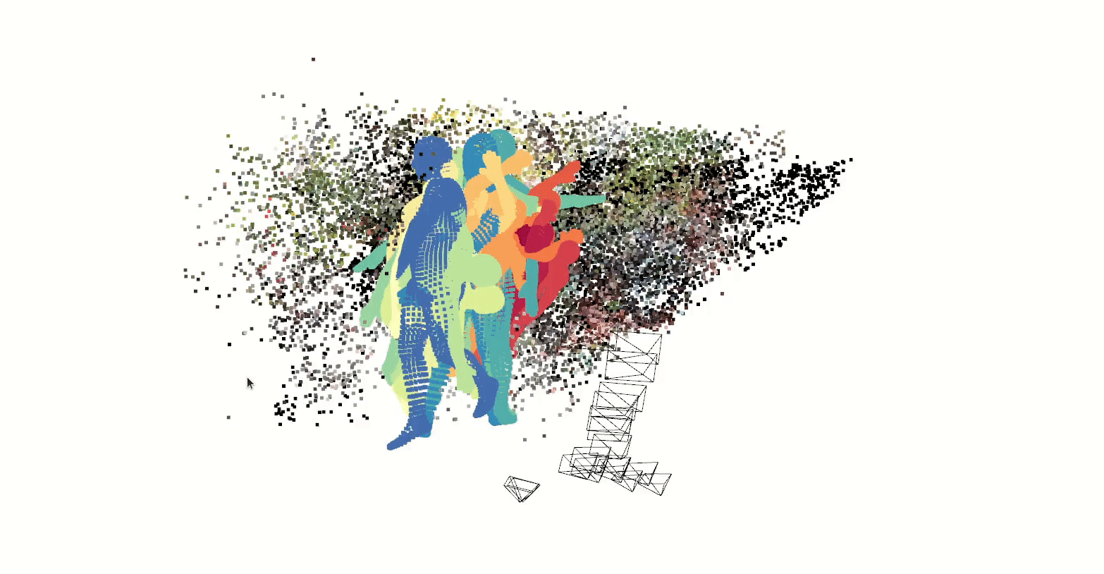
The newest version of BodyPix also features multi-person inference so we tried to recreate a Kali fight scene featuring two people. We took a video of ourselves trying to move like fighters with sticks. From this video, we extracted pose estimates, color coded for each individual, and used BodyPix for body part segmentation.
We found that using BodyPix in addition to pose estimation lets us transfer body shape as well as motion!
In this work, researchers introduce a semi-supervised learning formulation to disentangle the tasks of modeling motion and appearance for a target object class.
Then we can extract the keypoints from a driver video and use the appearance of a target image to produce motion transfer in one shot.
This means we don’t need to fine-tune a GAN for each individual! Instead, we can learn a motion model from a corpus of dancers and generate our motion transfer from a single image.
You can see the model lacks the same capacity to generate realistic images as StyleGAN variants, however, this technique applies to object classes which have no existing pose estimation model.
In last year’s post on generative models, we showcased theatrical posters synthesized with GANs and diffusion models.
Since that time, Latent Diffusion has gained popularity for faster training while allowing the output to be conditioned on text and images.
This variant performs diffusion in the embedding space after encoding text or image inputs with CLIP. By allowing the generated output to be conditioned on text and/or image inputs, the user has much more influence on the results.
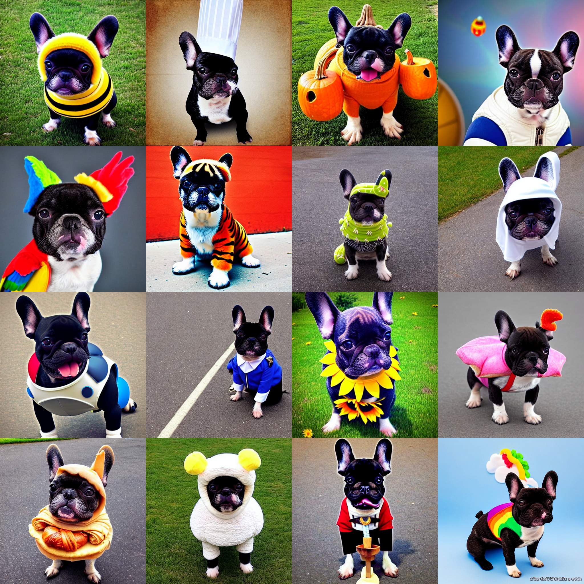
Fine-tuning these models, we created a virtual Halloween costume fitting for our dog, Sweetpea:
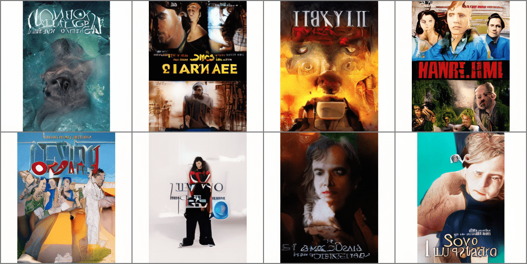
Next, we trained a latent diffusion model from scratch on our FilmGeeks movie poster collection:
Stability.ai trained Latent Diffusion on billions of images, using thousands of A100 GPUs before releasing the model as “Stable Diffusion”. This is free despite a total training cost in excess of $600K!
With these pretrained models, you can design a wide variety of prompts to evoke specific themes and aesthetics to generate custom content on-the-fly.
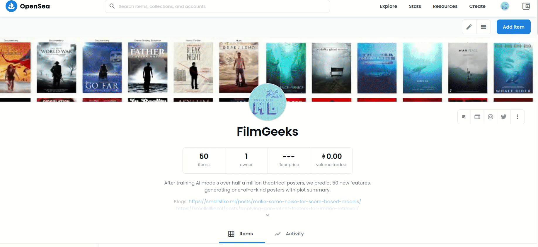
We try using stable diffusion to generate samples conditioned on custom prompts as well as the output of our filmgeeks latent diffusion model.
You can see our favorite samples in FilmGeeks3 on Opensea!
Besides making entertaining images, we experimented with applications like data augmentation. Similar to last year’s synthetic data experiment, we augment sample objects by performing “style transfer” to randomize the image texture before rendering novel perspectives using Blender/Unity.
Stable Diffusion supports transferring themes and concepts learned from a massive corpus of text-image aligned data scraped from the web. For example, we can synthesize a tattooed variant of our image texture above by conditioning on it as input along with a descriptive prompt:
Latent diffusion isn’t only for generating images. Motion Diffusion Models shows how we can synthesize realistic human motions described by the text prompt.
This can be used to articulate SMPL objects through motions that are not well-represented in activity recognition datasets. With 3D rendering, we can generate views from many different perspectives.
See our video on data augmentation with Latent Diffusion.
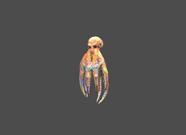
Finally, we mention that Latent Diffusion is being used to generate 3D assets as well as video. Using models like Stable Dreamfusion, you can generate 3D assets conditioned on a text prompt like our fish:
Check out some of our other samples on sketchfab:
Powerful, open-sourced models like Stable Diffusion make it easier and cheaper to access high-quality data for human or machine consumption.
Latent Diffusion has the power to condition samples on image and/or text which provides a lot of control in designing datasets specialized for your application.
We are excited to apply these techniques in content generation and few-shot learning from synthetic data.
Many recent successes in computer vision have been powered by the extension of BERTology beyond the mode of text-based data to image & video. Without a doubt, efficient Transformers which patchify input images a la ViT have initiated much of this progress. But in this post, we are interested in pretraining with self-supervised learning to develop compact representations we might use in various downstream tasks.
Datasets of real world interest often exhibit structures which are not exploited in research on benchmark datasets. Modeling around structures in the data, the ML practitioner can frame learning around auxiliary tasks with cheap supervisory signals. In practice, the robustness of deep learning to noisy labels makes this a reliable technique.
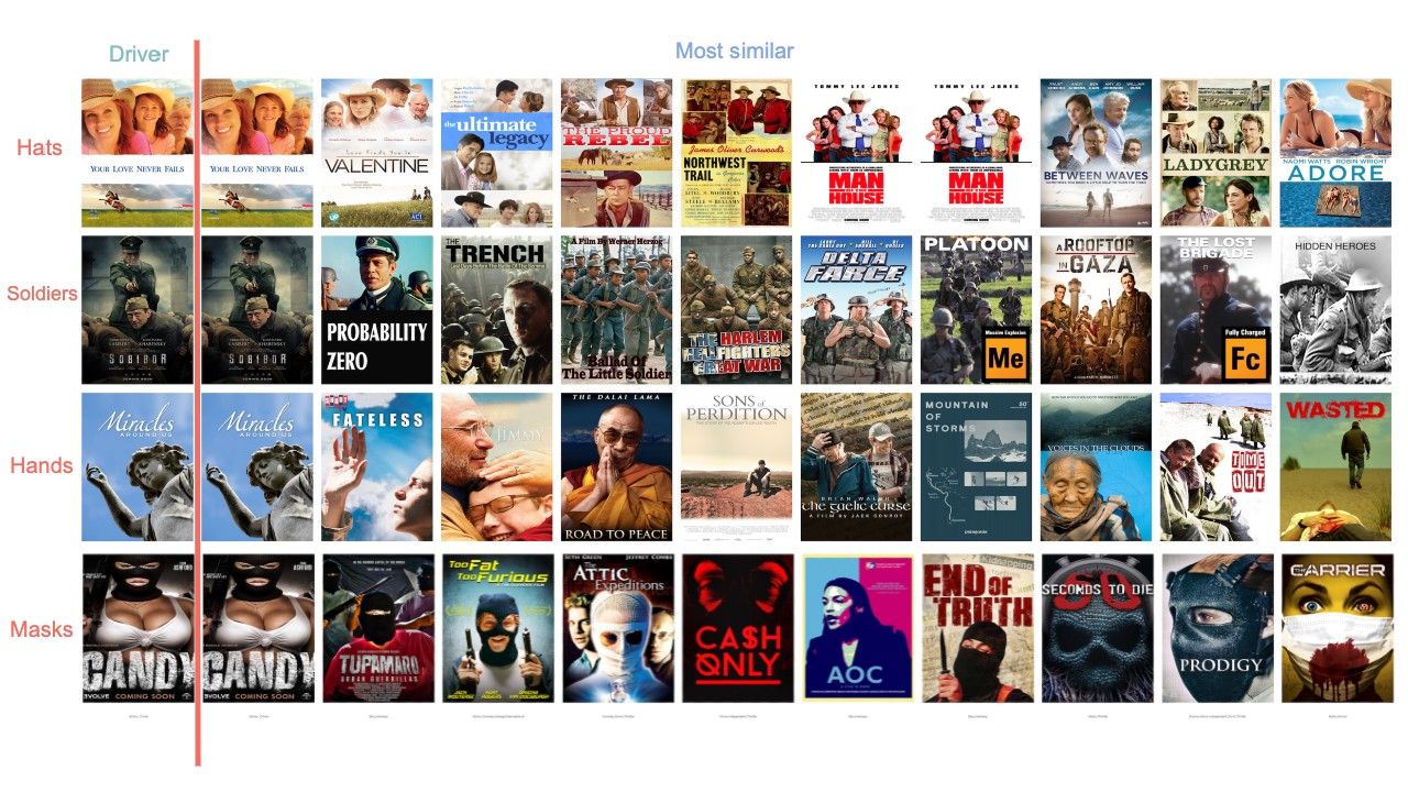
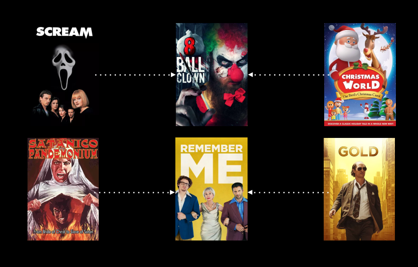
Indeed, we were surprised at the unreasonable effectiveness of coarse genre labels for developing representations for theatrical posters and applied fusion for a multi-modal extension to movie trailers.
But upon closer examination, we find much more structure in these human-generated compositions for human consumption. And in the case of content curated for humans, the cost of extracting more structure from an image corpus is relatively cheap.
We found openvino’s notebooks handy to quickly explore fast implementations of many models relevant to extracting more structure from our image corpus.
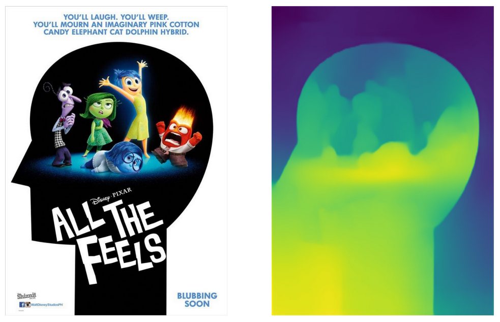
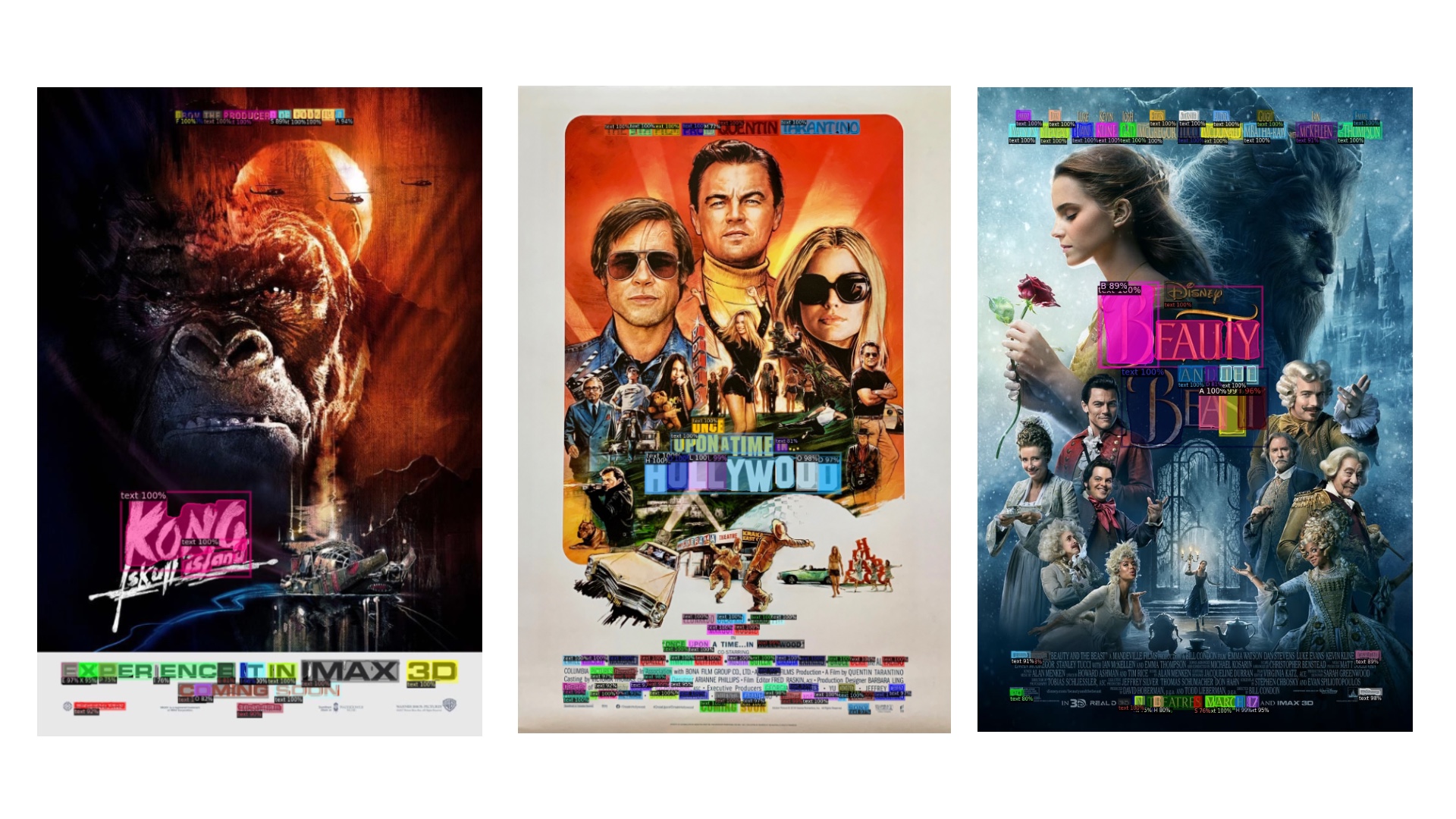
Our image corpus features layered compositions and these detection results can be leveraged to infer the title layer, but we can also use the text-based data to infer more information about the content with OCR.
Background segmentation offers another generally useful image processing technique we can use to analyze subjects in the foreground but our corpus provides especially challenging conditions we may need to work around.
With different perspectives, like monocular depth estimation, we can improve our estimation of saliency.
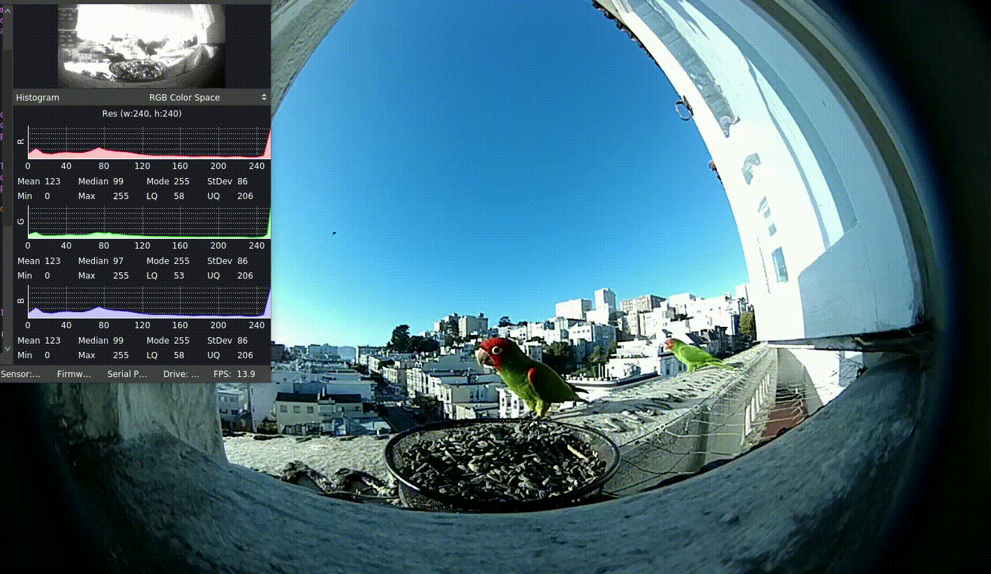
Depth information can even help reveal additional layers in the image compostions:
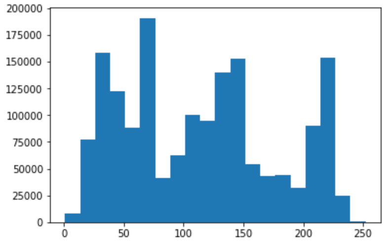
Looking for modes in the histogram of pixel intensities over the depth map, we might estimate 3 layers:
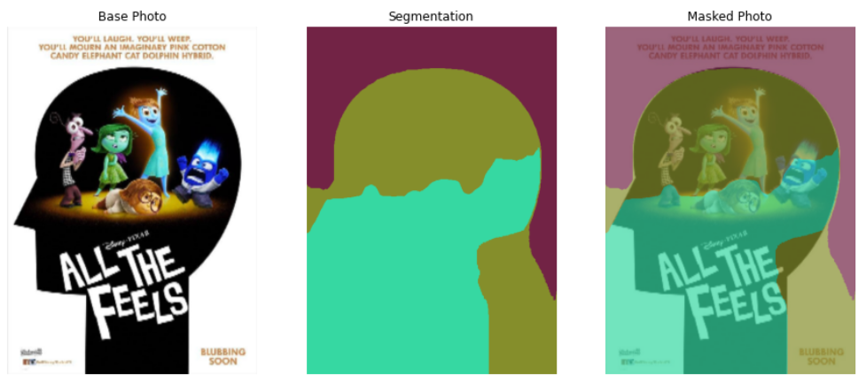
And after applying K-means (K=3), we find segmentations like:
Assuming we’ve performed OCR as above, simple heuristics guide our choice to label the green mask as the “Title Layer”. Trading off background segmentation with depth, and perhaps superpixel algorithms, we can focus additional analysis around the foreground subjects.
Simple featurizations of the foreground layer might include embeddings from image classifiers pre-trained on datasets like ImageNet or more structured pipelines using face or object detectors, perhaps with additional fine-tuning and even secondary models.
We’ve discussed numerous model-based inferences to acquire structured info about our image corpus. But sometimes, we can join additional sources like text or video data and attempt to fuse representations or apply cross-modal learning. PolyViT presents an exciting method of co-training a shared Transformer over multiple modalities of data.
After building up this rich structure, we can consider the different SSL tasks we can frame. SimSiam shows a simple approach using contrastive learning over pairs generated using alternative views of each image.
With layers and composition, as well as objects and text, we can frame all kinds of challenges for training. For example, we might consider the relationship between:
patches from foreground/background layers
salient objects among the foreground
text/font and image semantics
Our annotations go beyond genre labels, allowing us to develop our own labeling scheme for curriculum learning. For example, we might augment labels with metadata encoding info like title placement.
Conclusion
Structured signals are all around us and the flexibility and improved accessibility of deep learning makes it cheap to experiment in developing representations.
As architecture search converges around the use of Transformers, the tasks used in pretraining with SSL and the way they are staged allow the practitioner to to instill inductive biases relevant to the data.
While prototyping YogAI, our smart mirror fitness application, we dreamed of using generative models like GANs to render realistic avatars.
For the TFWorld 2.0 Challenge, we came a bit closer to that vision by demonstrating a pipeline which quickly creates motion transfer videos.
More recently, we have been learning about reconstruction techniques and have been excited about the work around Neural Radiance Fields (Nerf).
By this method, one learns an implicit representation of a scene from posed monocular videos. Typically, you start with video and use tools like colmap in order to align frames with camera poses.
The red markers indicate camera poses for each frame of a short video recording of glass figurines on a shelf.
With a trained nerf model, you can render novel views of the scene for a given input camera pose!
This last sequence was generated after training DSNerf, which supervises training with depth information we get for free by running colmap to process our input video. Adding depth-supervision to the loss aids model convergence while training on fewer samples.
Using simple scenes and limited perspectives, nerf can generate very realistic renditions. Next, we try a highly varied perspective of a complex, highly occluded scene of a figtree.
Less surprisingly, the rendition is not nearly as realistic as in the previous input scene.
Our latest experiment uses ml-neuman, decomposing a scene before applying nerf to represent a person.
For a successful rendition, we found it best to:
record in landscape mode and NOT portrait to avoid distortions
maintain a steady tracking shot with person in full FOV
train on a GPU with 24GB RAM
vary body position/orientation
Nerfs can render from many perspectives given relatively few training samples, which could have applications for sim2real in model training with synthetic data.
Some works focus on improvements using other supervisory signals or on making inference faster and we are excited to explore these developments as the technology matures.
Check out our repo for resources on hacking the Coral EdgeTPU dev board!
Earlier this year, Google released their Coral edgeTPU dev board! We were excited to get our hands on one and explore an embedded platform specifically designed for deep learning applications.
The Setup
Getting the dev board up and running wasn’t too complicated. It was somewhat different than setting up a pi with a raspbian image on a microSD card. However, we appreciated that the Google coral team provided different methods for setting it up.
The edgeTPU dev board requires a linux distribution, specifically Mendel Linux, to be flashed directly onto the board. With a microUSB port, you can communicate with the board via serial from any linux/OSX host machine and uses a USB-C port to transfer data and do the actual flashing. Their getting started instructions are simple to follow. Briefly, here are some findings while setting up the board:
Make sure you use a USB-C cable that can can also be used to sync when you connect it to the data (OTG) port on the device. This seems like a no brainer, but can be easy to forget and end up stuck not knowing why nothing is showing up on your screen.
Some report issues using a regular computer running linux or OSX and some recommend using a raspberry pi to aid in the flashing instead.
Flashing mendel onto the dev board got stuck trying to reboot correctly, so we found that the instructions they provide for reflashing your device when you’ve bricked it are really reliable! Also somewhat resembles flashing a raspbian distro onto an sd card for a pi.
The edgeTPU comes with a special API for running inference on the device. If you have played with TFLite, this is very similar as the API will use TFLite files for inference. Check out all the methods supported here!
The Google Coral team also provides an EdgeTPU compiler which lets you optimize a quantized tflite model for running inference on the dev board. For now, it only supports certain models for compilation. They also have an online version of the compiler if you don’t have a 64bit debian based linux computer. Their docs also provide excellent explanations on how the compiler works and all the methods available.
Testing Inference Speed
For one of our projects, YogAI, we used a raspberry pi 3 to run pose estimation as a feature extractor to feed to a simple classifier for pose classification. We found that on a non quantized, tflite model based on Convolutional Pose Machines got us around 2.5 fps. This was just enough to classify more stable poses like Yoga and some simple motion like squats vs deadlifts vs standing. But for better resolution on movement and overall perfomance, it would be great to see if another platform could speed up inference significantly. We used this model as a reference for comparison with aquantized tflite model compiled using the edgeTPU compiler.
Ildoonet’s tf-pose-estimation repo provides several pose estimation frozen graph models that we can quantize and convert to tflite. We chose a mobilenet based model since these are smaller and should perform well on small devices. To convert the frozen graph pb file found here, use the tensorflow 1.13.1 tflite methods from contrib like so:
This will produce a quantized tflite version of the model so we can then run it through the edgeTPU compiler. It is very simple to compile the file for the edgeTPU dev board. After installing or using the online version of the edgeTPU compiler, simply run:
From here, we’ll want to transfer the file over to our dev board! You can transfer data to the device by physically connecting to it via serial and the OTG port, but it is much nicer to be able to use ssh and scp to communicate with the device. There’s this nifty command-line tool that the Google Coral team has provided, mdt, that lets you open a shell, scp files around, and more. Follow the docs to install it on your host machine, connect to your dev board using the OTG port and run:
$ mdt shell
From your host machine, scp the compiled tflite model and a sample image to your dev board:
To run inference using the tflite compiled model, run this snippet:
from edgetpu.basic.basic_engine import BasicEngine
import numpy as np
from PIL import Image
import time
import argparse
if __name__ =="__main__":
default_model ='compiled_openpose_edgetpu.tflite'
default_image ="example.jpg"
parser = argparse.ArgumentParser()
parser.add_argument('--model', help='.tflite model path',
default=default_model)
parser.add_argument('--image', help='image file path',
default=default_image)
args = parser.parse_args()
'''load the image'''
target_size=(432, 368)
image = Image.open(args.image)
image = image.resize(target_size, Image.ANTIALIAS)
image = np.array(image).flatten()
'''load the model'''
engine = BasicEngine(args.model)
results = engine.RunInference(image)
print(engine.required_input_array_size())
print(results)
print('processing time is', results[0])
heat_map = results[1].reshape([54,46,57])
print('heatmap shape is',heat_map.shape)
print(heat_map)
print()
print()
print(np.sum(heat_map), (heat_map[1])
np.save('/home/mendel/heat_map.npy', heat_map)
When we run it on an example image, we’ve found that inference takes ~13 milliseconds, which is reaching ~77 fps! It’s an incredible speed up from simply running a tflite model on a pi. The board conveniently comes with an HDMI and USB port, so we can attach a screen and usb camera.
All in all, the edgeTPU dev board shows great promise for fast inference on the edge and can be used for all kinds of robotics applications. However, this requires installing various libraries that aren’t officially supported yet, since Mendel OS is not a mainstream linux distro. Installing tools like opencv, ROS, and proprietary camera SDKs took some tinkering to get right, so we created a repo with a few guides on how to install common libraries.
Finding similarities
We started by finding which linux distros were most similar to Mendel OS.
One way to do this is by looking at the libc and linux kernel:
# Looking at libc:
$ /lib/aarch64-linux-gnu/libc.so.6
GNU C Library (Debian GLIBC 2.24-11+deb9u4) stable release version 2.24, by Roland McGrath et al.
Copyright (C)2016 Free Software Foundation, Inc.
This is free software; see the source for copying conditions.
There is NO warranty; not even for MERCHANTABILITY or FITNESS FOR A
PARTICULAR PURPOSE.
Compiled by GNU CC version 6.3.0 20170516.
Available extensions:
crypt add-on version 2.1 by Michael Glad and others
GNU Libidn by Simon Josefsson
Native POSIX Threads Library by Ulrich Drepper et al
BIND-8.2.3-T5B
libc ABIs: UNIQUE
For bug reporting instructions, please see:
.
# Looking at kernel
$ uname -a
Linux undefined-calf 4.9.51-imx #1 SMP PREEMPT Tue May 14 20:34:37 UTC 2019 aarch64 GNU/Linux
It is apparent that Mendel OS is a Debian based distro and looking at the kernel, it is similar to Ubuntu 16.04 as this was its default kernel version. The architecture is aarch64 which is similar to ARM64. So whenever there are available packages for Ubuntu 16.04 for ARM64 architecture, we can probably install these on Mendel OS too. Looking at the Debian version gives us:
# Looking at Debian version
$ cat /etc/debian_version
9.7
This version translates to Debian stretch, which means that packages for raspbian stretch could also be compatible for Mendel OS.
The Google Coral Dev board makes running inference on device a lot faster, at times faster than running on a full server. Although it depends on a specialized flavor of Debian maintained by the Coral team, it is familiar enough to work with.
Check out the repo and enjoy the video on YogAI and ActionAI
Wanting a personal trainer to help track our fitness goals, we figured we could build our own. The goal was to build an application that could track how we were exercising and began with Yoga as a simple context. We dubbed our first iteration of this application as YogAI.
We thought about the YogAI concept for some time. Initially, we envisioned a smart yoga mat based on computer vision for corrective posture advice. We found out that others have taken the approach of embedding sensors within the yoga mat, although it appears they too are interested in vision.
We returned to the idea after seeing interesting work using pose estimation that we wanted to reproduce. However, we decided to put YogAI on a smart mirror platform.
By framing photos from the perspective of a large mirror on the wall rather than on the ground from a yoga mat upward, we could train models using yoga photos from the wild. These typically feature full body perspective from a distance at a height typical of a photographer.
Making a smart mirror is simple enough: just need an old monitor, a raspberry pi, and a one-way mirror, see how we built it here. We add a camera and microphone to support VUI and a visual analysis of the user, all taking place on-device.
To evaluate our concept, we begin by gathering images of Yoga poses with an image search for terms like: ‘yoga tree pose’, ‘yoga triangle pose’, etc. We chose yoga because the movements are relatively static compared to other athletic maneuvers, this makes the constraints on frame rate of inference less demanding. We can quickly filter out irrelevant photos and perhaps refine our queries to build a corpus of a couple thousand yoga pose images.
We’d love to achieve the speed of a CNN classifier, however, with only a few thousand images of people in different settings, clothing, positions, etc. we are unlikely to find that path fruitful. Instead, we turn to pose estimation models. These are especially well-suited to our task of reducing all the scene complexity down to the pose information we want to evaluate. These models are not quite as fast as classifiers, but with tf-lite we manage roughly 2.5 FPS on a raspberry pi 3.
Pose estimation gets us part way. To realize YogAI, we need to add something new. We need a function that takes us from pose estimates to yoga position classes. With up to 14 body keypoints, each of our couple thousand images can be represented as a vector in a 28-dimensional real linear space. By convention, we will take the x and y indices of the mode for each key point slice of our pose estimation model belief map. In other words, the pose estimation model will output a tensor shaped like (1, 96, 96, 14) where each slice along the final axis corresponds to a 96x96 belief map for the location of a particular body key point. Taking the max of each slice, we find the most likely index where that slice’s keypoint is positioned relative to the framing of the input image.
This representation of the input image offers the additional advantage of reducing the dimensionality of our problem for greater statistical efficiency in building a classifier. We regard the pose estimation process as an image feature extractor for a pose classifier based on gradient boosting machines, implemented with XGBoost.
Then we were able to quickly demonstrate our approach by training a gradient boosting machine. It didn’t take much parameter tweaking before we were able to evaluate our pose estimation model.
Shortly after, the proof of concept got covered in MagPi Magazine!
It was natural to consider how we might use pose estimates over time to get a more robust view of a figures position in the photo. Having built a reasonable pose classifier, this also begs the question how we might generalize our work to classifying motion.
Our first idea here was to concatenate the pose vectors from 2 or 3 successive time steps and try to train the tree to recognize a motion. To keep things simple, we start by framing a desire to differentiate between standing, squatting, and forward bends (deadlift). These categories were chosen to test both static and dynamic maneuvers. Squats and Deadlifts live on similar planes-of-motion and are leg-dominant moves though activating opposing muscle groups.
We found a couple youtube videos of high repetition moves performed by fitness athletes filmed from a perspective similar to the design of our smart mirror. We split the videos using ffmpeg and ran pose esimtation to get our pose vector representation of each frame after some minor edits to cut out irrelevant video segments.
Our gradient boosting machine model seemed to lack the capacity to perform reasonably. We decided to apply LSTMs to our sequence of pose vectors arranged in 28xd blocks, sweeping d in {2, 3, 5}. After some experiementation, we determined that 2 LSTM blocks followed by 2 fully connected layers on a 28x5 input sequence yielded a reasonable model.
Now we have basic motion classification!
Introducing ActionAI
Advancements in edge devices specialized for machine learning training/inference on device and various machine learning libraries improving inference time on pose estimation models gave way for improvements in FPS for classifying poses and movement.
We abstracted the technique of using pose estimation inference output as input for an LSTM classifier into a toolkit called ActionAI. It’s prominently feaured in GitHub’s human action recognition topic and received a prize in NVIDIA’s AI at the Edge Challenge!
ActionAI generalizes the approach of YogAI and related projects framing an IVA pipeline by introducing trackers and multi-person pose estimation.
By baking pose estimation into the pipeline as the primary inference engine, the developer can focus on training simple image classification models based on low dimensional features or small, localized image crops.
Since popular IVA frameworks typically only support the most common computer vision tasks like object detection or image classification/segmentation, we needed to implement our own.
Many IVA frameworks use GStreamer to acquire and process video. For our video processing demo, OpenCV suffices. For pose estimation we use Openpose implemented with popular deep learning frameworks like Tensorflow and Pytorch.
Accurately recognizing some activities requires higher resolution in time with higher frame rates, so we use TensorRT converters for optimized inference on edgeAI prototyping devices like the Jetson Nano.
The main programming abstraction of ActionAI is a trackable person class, similar to this pyimagesearch trackable object. This object has a method to enqueue the configuration of N (14 or 18) new keypoints as a length 2N numpy array into a circular buffer. For computational efficiency, we prefer smaller buffers, but we balance this desire with one to provide enough information as input for secondary models. This object also encapsulates ids, bounding boxes, or the results of running additional inference.
To track person instances, we used a scikit-learn implementation the Kuhn–Munkres algorithm based on the intersection over union of bounding boxes between consecutive time steps. This blog has nice exposition on applying this algorithm to perform matching.
Like other IVA frameworks, we incorporate visual overlays to support ML observability and introspection as well as visual storytelling.
In another direction, by polling for button presses of a PS3 controller connected to the Jetson Nano by USB, we easily annotated activities for person instances at each time step interactively, like we did with the MuttMentor.
This makes an ideal prototyping and data gathering platform for Human Activity Recognition, Human Object Interaction, and Scene Understanding tasks with ActionAI, a Jetson Nano, a USB Camera and the PS3 controller’s rich input interface.
In YogAI, we found sequences of pose estimates to be powerful features in recognizing motions from relatively few samples. In ActionAI, by running model update steps inline with image acquisition and PS3 controller annotation, we can implement a demo similar to the teachable machine.
We hope by sharing this toolkit, others are more easily able to classify their own set of actions at the edge. Some have suggested using ActionAI for identifying their karate katas or dance.
In our last post, we trained StyleGAN2 over a corpus of hundreds of thousands theatrical posters we scraped from sites like IMDb.
Then we explored image retrieval applications of StyleGAN2 after extracting embeddings by projecting our image corpus onto the learned latent factor space.
Image retrieval techniques can form the basis of personalized image recommendations as we use content similarity to generate new recommendations.
Netflix engineers posted about testing the impact on user engagement from artwork produced by their content creation team.
Without a design team, we seek algorithmic methods to generate variants. Many of our variants are merely near-duplicates, differing only by aspect ratio or otherwise minor details.
In this post, we apply generative models to create content for producing localized image variants for recommendations.
Localization
Before considering fully personalized image recommendation, we can explore regional variants through localization.
Here, “localizing” image content means replacing the text-based title overlays of an image with one rendered in the regional lingua franca.
Since we scraped our corpus, we lack the original creatives and must instead apply some image edits.
Specifically, we want to mask out the region of the theatrical poster with the title text. Then we want to insert the new localized title variant.
After masking out the title, we must blend backgrounds to maintain similar production quality for our poster.
While simple enough for a few posters, scaling this work for dozens of language variants over a catalogue of thousands or more items with multiple images variants is infeasible.
The prohibitive cost of hiring a design team along with the lack of variants can limit greater image personalization, so we want to automate this as much as possible.
Our ML Application
We can decompose our goal of poster localization into the following steps:
Identify regions of interest containing title text
Mask out these regions
Apply image inpainting
Add new localized overlay
Text Detection
To detect titles, we tested text detection models like EAST, but theatrical posters can be complex compositions so we look for newer, more accurate models.
Surveying scene text detection on paperswithcode, we found TextFuseNet to be a powerful and fast detector for image compositions.
After detection, masking is straightforward and sets us up for the crux of this problem, blending the new overlay into the original image.
Image Inpainting
Upon annihilating the image regions containing text with a mask, we apply image inpainting to approximate the original background image.
Turning again to paperswithcode, we find SOTA references in the domain of image inpainting dominated by GANs.
This model uses the StyleGAN2 latent factors we learned before as priors in a Bayesian model and the results are quite compelling.
Conclusion
After learning StyleGAN2 representations of our poster corpus, we can support image personalization by generating greater variation in our content with automated image editing techniques.
Image editing tools aided with data-driven priors can enable large scalable design workloads by nonexperts.
title: “IVA Pipelines with NVIDIA TLT and Deepstream SDK 5.0”
date: 2020-05-08T18:00:00-07:00
tags: [‘computer vision’, ‘Jetson’, ‘tensorflow’, ‘video’]
draft: false
We have seen applications in industries like retail, telemedicine, and robotics enabled by video analytics with machine learning. ML practitioners often leverage transfer learning with pretrained models to expedite development. Computer vision applications can benefit from using video analytics frameworks to facilitate faster iteration and experimentation.
NVIDIA’s TLT toolkit and the Deepstream SDK 5.0 have made it easy to experiment with various network architectures and quickly deploy them on a NVIDIA powered device for optimized inference.
To experiment with these new software, we used the TLT toolkit to fine tune a detectnet_v2 model on a fashion dataset to detect dresses, jeans, and tshirts. Then we used the new Deepstream SDK 5.0 to deploy the model on a Jetson device for a smart personal wardrobe assistant we nicknamed Stilo.
NVIDIA has released a docker container with TLT configured and includes a directory of jupyter notebooks with examples on how to fine-tune various model architectures from their model zoo.
Following the detectnet_v2 example notebook includes all the config files needed to properly train, prune, retrain, and deploy a model.
Train
To train, we used the GPU configuration:
It’s also very easy to visualize the results for a quick sanity check:
Prune
Next we prune our model. Pruning helps reduce the memory footprint of the model and increases inference speed.
Retrain
Next, we retrain the pruned model, bumping up the performance of our model by almost 10%!
Deployment with the Deepstream SDK 5.0
The Deepstream SDK was designed to help developers build high-performance, machine learning based real-time video analytics applications. It is as simple to use as the TLT toolkit, boiling down to editing a few config files and running the command line interface.
The SDK also comes with lots of examples on how to deploy multiple models, with a variety of inputs (file, camera) and outputs (file, RTSP Stream). Since the SDK is based on GStreamer, it is flexible on input and output interfaces it can process.
Deploy
We used an example from the tlt pretrained model config examples found in /opt/nvidia/deepstream/deepstream-5.0/samples/configs/tlt_pretrained_models.
We simply added a label file with our three categories:
# in a file called labels_fashionnet.txt
dress
tee
jeans
You can take an example config_infer_primary file like config_infer_primary_peoplenet.txt and point to you model assets:
# modify the following:[property]
tlt-encoded-model=<TLT model>
tlt-model-key=<Key>
labelfile-path=<Label file>
int8-calib-file=<INT8 Calibration cache>
input-dims=<Inference resolution>
num-detected-classes=<# of classes>
Finally, we copied an example deepstream_app_source1 file from the peoplenet example to point to our new config_infer_primary file above.
[primary-gie]# near the bottom of the section
config-file=config_infer_primary_fashionnet.txt
Now just run deepstream-app -c deepstream_app_source1_fashionnet.txt.
The TLT toolkit and Deepstream SDK simplify training and deployment of models optimized for streaming video applications. Prototyping IVA applications can be reduced to modifying configuration files.
For our prototype, this helped us quickly evaluate a real world video stream. To improve performance, we would add more training samples that look closer to our deployment scene inside a closet.
Like others, we’ve noted a recent uptick in research implemented using Jax. You might chalk it up as yet another ML platform, but Jax is emerging as the tool of choice for faster research iteration at DeepMind.
After exploring for ourselves, we’re excited to find Jax is principally designed for fast differentiation. Excited because differentiation is foundational to gradient-based learning strategies supported in many ML algorithms. Moreover, the derivative is also ubiquitous in scientific computing, making Jax one powerful hammer!
A Whiff of AutoDiff
We found this excellent survey on automatic/algorithmic differentiation (autodiff) and differentiable programming quite illuminating.
Recall back in calculus, we conceptualized the derivative as a limit of successively better approximations to the tangent space of a function at a point. This perspective motivates numerical differentiation techniques like the finite difference method. The convergence of these methods is challenged on the one hand by sensitivity to choice of step size and the other by an accumulation of round off errors.
A little further into calculus, we learned simple rules for differentiating algebraic and transcendental functions. We learned how the derivative interacts with function composition as well as other operators like the sum and product. These insights shaped symbolic differentiation techniques used in tools like Mathematica. Unfortunately, this approach suffers from an explosion of terms when computing derivatives for function compositions, no good for deep learning.
Jax takes a different tack with autodiff. This endows Jax with the ability to translate your code into certain primitives for which the derivative is known, akin to symbolic differentiation. Crucially, these primitives include control flows like branching and looping, making it simple to just apply the dang derivative.
Unlike symbolic differentiation, autodiff uses a computation graph to efficiently determine and accumulate function values and derivatives. With respect to the computation graph’s topological ordering, we consider forward and reverse mode AD. Deep learning practitioners are already familiar with backpropagation, which can be realized as reverse mode auto differentiation.
Just the gist of jit, xla, vmap
The Jax compiler optimizes high-level code for xla by way of a statically-typed expression called a jaxpr. Jax naming and typing help to manage complex, structured data through the pytrees api.
The Jax transformation model emphasizes pure functions, implying some consideration required for handling stateful computations.
Jax can trace a program with jit to generate fused operations over reduced-precision numeric representations optimized for hardware accelerators.
Jax is designed to easily support the data and model parallelism used to efficiently scale up training of ML models. Vectorizing a transformation is trivial with vmap.
Jax Docs Rock!
The official documentation is full of demos highlighting the unique capabilities of the tool!
For instance, with easy, scalable differentiation, you can wrangle nonlinearity by implementing fixed point solvers using the vector-jacobian product or even make a custom VJP for integration over a riemannian manifold.
This example shows how temporal-difference updates can be cast as derivatives of a pseudo loss function while using Jax’s fine-level control of gradient computations to tackle problems in RL.
A favorite example generates images after learning the vector field arising from the gradient of log data density p(x) w.r.t x. Learning is accomplished by annealing the amount of perturbative noise applied to examples during training. In the end, randomly initialized points can seed trajectories which flow along the vector field to iteratively refine generated samples via Langevin dynamics!
Lately, I’ve been revisiting studies in scientific computing and machine learning to consider innovations at the intersection of these disciplines. Perhaps Jax will accelerate the convergence of ML & scientific computing with an abstraction that appropriately elevates the derivative.
We’re just getting started but Google makes it easy to borrow TPUs so you too can join us in a jaxtragavanza of experiments in computing this Summer!
Factors like cheaper bandwidth and storage, expanded remote work, streaming entertainment, social media, robotics and autonomous vehicles, all contribute to the rapidly increasing volume of video data.
Nonetheless, performance in benchmark ML video tasks in perception, activity recognition, and video understanding lag behind the image counterpart.
In this post, we consider the challenges in applying ML to video while surveying some of the techniques en vogue to address them.
The Time Dimension
Treating video analytics as a search over space and time, the dimensionality begets additional hurdles to statistical and computational efficiency. Video inherits the HxWxD pixel grid from the image domain while extending dimensionality into the time dimension!
General video multimedia streams may feature multiple video or audio tracks. For our purposes, we consider video as a sequence of image frames sampled in time.
Each frame is associated with a timestamp at capture which imposes a natural sequential ordering of frames, often referenced by index. By probing, we find the average frame rate at which a multimedia container plays, measured by frames-per-second (fps ~ hertz).
Typically video is recorded at a resolution sufficient to smoothly resolve the position of a subject in time. This may afford the opportunity to eliminate computations of slowly-varying or uninteresting content without adversely impacting temporal consistency using simple strategies like skipping frames.
Motivated by results of Shannon, we recognize that complex and highly-variable video demands more samples in time to adequately characterize.
Spatial Dimensions
Computer vision tasks like segmentation benefit from higher spatial resolution input for fine-grained predictions. However, characterizing an image globally via classification typically utilizes lower frequency features like color and shape, hence can be efficiently computed over smaller images.
Analogously, spatial resolution requirements for video vary by application from high-fidelity cinematic or scientific content to low-resolution user-generated content optimized for serving.
For statistical and computational efficiency, spatial information can be coarsened from pixel level data since video features objects which are spatially similar in a local sense.
Geometric priors including shape and distance offer powerful signals to parse information from video. Using these spatial regularities we can pass to sparse, pointwise information while inferring global structure.
As with images, we frequently observe a center bias in the framing of subjects in video. Space reduction strategies range in simplicity from center cropping to introducing the context of saliency or key points. Even semantic object detection can be employed to specify regions of interest, localizing video for streamlined computations.
Localizing in Space
A module to identify and track object instances over time is important to characterize events in a video stream. Most tracking algorithms match objects to candidate region proposals over time by visual similarity or with a motion model.
In this databricks notebook, we implement a pyspark Transformers for face detection and tracking.
Localizing in Time
Object tracking heuristics can break down in complex, edited video sequences demanding additional processing to extract disjoint segments where these assumptions still hold. In a previous post we demo shot detection with Spark + FFmpeg.
For short and simple shots, sparsely sampling frames may suffice to represent the segment. We found this to be the case for modeling content-based video similarity models in prior experiments.
Offline v. Online Processing
For real-time applications, hardware-optimized implementations of simple models distributed closer to the source of capture can be performant. Search and anomaly detection tasks can use fast models to associate frames with a stream of annotation data.
Also user-generated content may be too voluminous to run complex inference workloads. Here fast, simple representation to index the catalogue can help.
Conversely, a slowly-growing corpus of curated cinematic content tends to present rich structure we can parse with additional modeling and analysis. Google offers a service to analyze and index metadata in video. Stanford researchers demonstrate vision pipelines for extracting structured information from video:
Pairing tools like Spark and FFmpeg, we can apply MapReduce to distribute processing the high-bandwidth sequential data. Here, we combine Spark with off-the-shelf face detectors, similar to the approach described above:
Popular video datasets used to benchmark video understanding & activity recognition tasks, including UCF101, Kinetics, and YouTube8M.
Youtube Downloader is fantastic for fetching a few videos, but it can be challenging to download a large corpus from YouTube.
The Deepfake Detection Challenge, hosted by Kaggle, provides a corpus of video data for the binary classification task of identifying videos manipulated by Deepfake techniques.
ML Models on Video
During the DeepFake Detection Challenge, many participants sampled frames from short video segments and ensemble the results of an image classifier for prediction. Some considered LCRN models using temporal sequences of features extracted from image patches around the face.
Similarly, we’ve encoded motion using sequences of low-dimensional body key points for activity recognition with ActionAI.
This survey outlines research advances introducing temporal information through the two-stream networks using RGB and optical flow as input along with its modern incarnation in the neuro-inspired Slowfastarchitectures. The survey considers different approaches regarding time, including 3D convolution as well as the recent emphasis on making video inference more efficient.
Qualcomm researchers recently applied conditional computing to reduce work over space-time volumes by apply convolution to sparse residual frames while learning to skip frames with a gating mechanism. Naturally more time frames can help some predictions.
We are excited to apply ideas like these for content-aware video compression techniques.
Conclusion
Inferring structured information from video is challenging. Simply storing and accessing suitable training samples or learning specialized tools can limit the broader application of this technology.
Video understanding presses the limits in extracting structure from high-dimensional data. Success in this arena draws upon advances in hardware acceleration and signal processing.
title: “Make Some Noise for Score Based Models”
date: 2021-07-02T12:33:34-07:00
draft: false
tags: [“differential equations”, “deep learning”]
Blob Pitt's next big blockbuster
We consider generative models among the most exciting applications of machine learning. This tech has reached a remarkable capacity to synthesize original multimedia content after learning a data distribution.
In this arena, the state-of-the-art has been dominated by a family of models called generative adversarial networks or GANs.
However, GANs are challenged by training instabilities. The latest StyleGAN2-ada mitigates mode collapse arising from overfit discriminators using test time data augmentation.
We’ve recently explored another exciting SOTA family of image synthesis techniques called score-based generative models. Under this model, training data undergoes a diffusion process so we can learn the gradient of the data distribution.
$$
\nabla_\mathbf{x} \log p(\mathbf{x})
$$
Now with an estimate for the gradient of the data distribution, we can perturb any point in $R^D$ to one more likely given the training data. This estimate provides a tool for model practitioners to evolve randomly initialized points under the flow prescribed by the learned vector field.
These diffusion processes can be expressed generally using the stochastic differential equation:
$$
\begin{align*}
d \mathbf{x} = \mathbf{f}(\mathbf{x}, t) d t + g(t) d \mathbf{w},
\end{align*}
$$
Framed this way, sample generation relates to the reverse time dynamics of such diffusion processes. Fortunately, researchers can apply Anderson’s result in stochastic calculus from the 80s to consider this reversal.
Cheaply sampled Gaussian initial conditions are used to generate realistic instances after evolving according to the learned “probability flow”.
Despite apparent similarities to normalizing flows, score-based models avoid the normalization challenge of computing high-dimensional integrals.
In fact, highly-optimized ODE solvers utilize the learned score vector field to generate samples by solving an initial value problem. Researchers also explored various sampling methods to improve the result quality, offering a nice template for extensions.
These computations leverage an approximation of the probability flow ODE using the related ideas of neural ODEs. Many of the models made an original debut generating realistic images in Denoising Diffusion Probabilistic Models.
Generating Custom Movie Posters with Score-based Models
The repo trains score models using Jax while making use of scipy ODE solvers to generate samples. The authors offer detailed colabs with pretrained models along with configurations referenced in their ICLR 2021 conference paper.
This makes it easy to generate realistic samples of CIFAR10 categories:
For rough comparison to previous experiments, we start by applying this generative model to a corpus of 40K unlabeled theatrical posters augmented by horizontal reflection. For training, we package the posters into tfrecords using the dataset_tool.py found in the StyleGAN2-ada repo.
Next, we try applying the high resolution configuration configs/ve/celebahq_256_ncsnpp_continuous.py used to generate results from CelebA-HQ to our theatrical poster corpus. This entailed restricting batch sizes to fit the model and training samples into GPU memory. Unfortunately, without shrinking the learning rate, this seemed to destabilize training:
Then, using the smaller model of configs/vp/ddpm/celebahq.py and reducing image resolution, we found samples generated over the course of training like:
Training 100 steps takes approximately 1.5 mins saturating 2 Titan RTXs but less than 15 seconds on 8X larger batches using TPUs!
With a promising start, we scale up training with an order of magnitude more images, including genre labels for class conditional training and generation, we find a qualitative improvement in the images synthesized.
Compared to experiments with StyleGAN2, we find greater variety in qualities like hair, gender, and facial expressions.
Conclusion
Fantastically, by corrupting training samples through a diffusion process, we can learn to approximate the reverse time dynamics using ODE solvers to generate realistic samples from noise!
We’ve even minted a selection of generated posters on OpenSea!
Cascaded Diffusion Models extend this line of work with a sequence of score-based models to progressively sharpen and resolve details of images generated by earlier steps in a cascade.
In this post, we share one of our favorite “pet projects”.
We first heard about the “parrots of telegraph hill” looking for things to see in the city. But after a couple years, we never managed to run into one of these accidentally re-wilded parrots.
Eventually, we moved to a new apartment where we could hear their distant squawks and occassionally see a small flock of the cherry-headed conures. Then, we began to notice a shadow going by the window and figured out that a pair of parrots were actually roosting next door!
Despite living so close, it was difficult to get a good view. Everytime we approached the window, they would take off so we set up cameras to view them without the disturbance.
In time, we earned their trust by putting out bird seed, even being able to hand feed them apples.
But these little parrots have good reason to be on guard as raptors are always on patrol.
Besides the safety in numbers, these birds are pretty good at disguise!
After much observation, we learned to recognize each by their markings and behavior.
Finally, as the chirps emanating from the nest grew louder, we even had the chance to spot a chick!
At the same time, we were inspired by the perspectives of modern animal documentaries, which have been greatly enhanced by embedded cameras. We dreamed of the views these animals must enjoy of our city!
Fascinated by these critters, we tried getting closer with embedded cameras like the arduino portenta.
We also set up depthai cameras with wide angle lens to detect & track our parrots.
With our feathery muses, we explore fast detection from the arduino.
Using the depthai camera, we can measure distance by calculating depth from stereo disparity.
But with a 7.5 cm baseline, we needed to try something else if we want to estimate distances greater than a few meters.
Recently, we’ve been experimenting with multi-view stereo especially using wide baselines. After searching around, we devised a plan to add long-range stereo vision for early bird detection.
Refer to Learning OpenCV for more details about calibrating stereo cameras. Generally, one performs calibration with a checkerboard but instead we use Hartley’s method and find keypoints with SIFT.
At a high level, by identifying points from each view, we can estimate the difference in camera pose. From this info, we can find the homography which warps one view to align with the second. This simplifies a search to match pixels and calculate the disparity which we use in reconstruction.
By adding a second 4K camera we can extend the depth range by tens of meters with a baseline as wide as a bay window!
Even though we can estimate distance at longer ranges, detecting our stereo parrots is still quite difficult! But researchers are applying similar techniques to protect migrating birds from wind farm turbines.
Up close, they are recognizable by the distinctive red-green pattern but at a distance, color is less discernable.
Instead, we humans recognize the parrots by their distinctive call as well as their shape and motion as they fly. We can try temporal stacking of three successive greyscaled frames as done to detect birds in flight.
In Chapter 12 of Learning FPGAs, the author guides us in building a sound direction detector with an array of microphones! We can add this component to focus our multi-camera system.
We’ve also been experimenting with visual servoing using a pan-tilt-zoom camera for tracking.
Perhaps we can use sound direction detection to focus our PTZ camera or make use of the Skagen & Klim datasets for more powerful parrot detection. Stay tuned for updates!
title: “Model Explainability With GradCAM”
date: 2021-08-24T10:45:03-07:00
Though accustomed to evaluating ML models with respect to performance statistics like accuracy, real-world deployment scenarios must weigh multiple models performing comparably. Deciding which to launch in A/B experiment can be challenging when the offline metrics are just a proxy for online metrics core to business decisions. Experiment time is precious and for large experiments on foundational models, the tolerance for error is limited hence it is critical to base experiment launch decisions on a collection of diverse metrics.
In computer vision, attention mechanisms feature the ability to explain model predictions by visualizing attention maps. In this post, we highlight a similar technique which generalizes to other CNN based architectures, called GradCAM.
Researchers at the Georgia Institute of Technology introduced GradCAM to help explain CNN model predictions. CAM stands for Class Activation Mapping, hinting at the mechanism of discriminating regions in the receptive field based on data labels.
By analyzing the gradient flow for a sample, CNN feature maps give rise to heat maps after a ReLU activation filters pixels not correlated with correctly predicting the label. Keras docs reference a simple implementation.
When making decisions about complex models, it helps to have a view into which factors influence model outcomes. As the researchers point out, model interpretability is important for building ML systems we can trust. Pairing GradCAM with mechanical turks provides a powerful comparison in how humans and algorithms reason about labeling example instances.
Additionally, GradCAM activations can be quantitatively compared to human attention via “the pointing game” referenced here
The researchers also show how GradCAM can be applied to identify bias in model performance to improve model fairness. In their proof of concept, they use these activation mappings to show models making decisions based on spurious reasoning due to bias in training samples.
These visualization techniques can even help develop counterfactual explanations for a sample, whereby we visualize regions most likely to change a network’s decision.
Seeking additional insights into our genre classifiers, we visualize some activation maps for theatrical posters.
Superimposing the heatmaps over the original images, GradCAM highlights regions of each sample important for genre prediction. While these heat maps appear to highlight relevant semantic content for predicting genres like sports, we are mindful of the potential bias in allowing convnets to focus on text.
Depending upon the context, it could make sense to provide the model with this information, perhaps even more directly. Still in another contexts, a model may overfit to information like this and lack robustness to variance in a title’s language. In this case, we could consider scene text removal similar to this demo.
The use of streaming services has sharply increased over this past year.
Many video streaming platforms prominently feature theatrical posters in content representation.
As movie posters are designed to signal theme, genre and era, this representation strongly influences a user’s propensity to watch the title.
Domain experts have remarked on how poster elements can convey an emotion or capture attention.
Exploring this thesis, Netflix conducted a UX study, using eye tracking to find that 91% of titles are rejected after roughly 1 second of view time.
In this project, we develop models to learn movie poster similarity for applications in content-based recommendations.
Genre information and Weak Labeling
In poster design, genre is often conveyed through low-level information like color palette in addition to higher-level structural and semantic indicators. For instance, an actor’s uniform may indicate the movie is about baseball.
Though easy to frame a classification task by aligning a title’s poster with genre labels, we ultimately seek embeddings transcending these labels to capture semantic similarity.
Metric Learning
Some describe using learned embeddings from the penultimate layer of a multilabel classifier as a representation for movie posters. In fact, Pinterest researchers find this approach performing on par with metric learning approaches.
However, this recently open-sourced module simplifies setting up metric learning tasks using weakly labeled images. This loss is more directly optimized for the task of measuring image similarity and it trivializes mining suitable triplets and learning with a margin-based loss.
Putting it Together
Movie posters are relatively complex compared to some image datasets like MNIST or FashionMNIST.
Qualitatively, we consider the complexity of this dataset between that of FashionMNIST and ImageNet. Therefore, we apply transfer learning from base networks pre-trained on ImageNet. Characterizing the intrinsic dimensionality of our movie poster dataset can be put on more precise quantitative footing using entropy measures like these researchers showed.
We also explore a warmup phase of fine-tuning a genre classifier before changing loss for metric learning. In this way, we initially compile with the keras.losses.BinaryCrossentropy(from_logits=True) loss.
We also found it helpful to progressively unfreeze lower blocks over the course of several training epochs using a method like this:
self.blocks = ["_18"]
deffreezeAllButBlocks(self):
self.model.trainable =Truefor i, block in enumerate(self.model.layers):
if block.name =="NASNetLarge":
ifnot self.blocks:
block.trainable =Falseelse:
for l in block.layers:
ifnot l.name.startswith(tuple(self.blocks)) or \
isinstance(l, layers.BatchNormalization):
l.trainable =Falsereturn self.model
Ultimately, we find higher capacity pretrained base network architectures like NASNet most performant. After this preliminary burn-in phase, we extract the model up to the logit layer with:
Incorporating the angular loss and following the guidance of these researchers, we tune the margin parameter for the dataset. We found smaller values of angular margin helpful: tfa.losses.TripletSemiHardLoss(distance_metric="angular", margin=0.1).
Combining these techniques helps to map semantically-related content to neighborhoods in an embedding space.
Finally, we can use simple candidate generation techniques like (approximate) nearest neighbors to recommend titles based on a historical interest indicated in a user’s watch history. Alternatively, we can use a ScaNN layer from tf-recommenders.
Results
Generating the top 10 most similar posters for sample queries, we find embeddings which transcend their genre labels to yield semantically cohesive neighborhoods.
Similar to word2vec, we can mix stylistic elements of posters by finding images near the averaged embedding.
Groups like Pinterest show that visual content-signals can be leveraged to help users discover relevant content.
By encoding semantic information presented in image content, we can more easily utilize the relatively abundant click through data to model user interests and behaviors to build more sophisticated recommender systems.
Though image classification has been shown to perform well for image retrieval and similarity, metric learning is easier than ever with Tensorflow’s TripletSemiHardLoss and more directly optimized for the task at hand.
Representation collapse poses a challenge in applying metric learning, whereby distinct inputs are mapped to the same output embedding by the model, ultimately failing to encode visual similarity. We find genre labeling of theatrical posters cheap and flexible while providing hard negatives to limit collapsed representations.
In a previous post, we discussed scraping a movie poster image corpus with genre labels from imdb and learning image similarity models using tensorflow.
In this post, we extend this idea to recommend movie trailers based on audio-visual similarity.
Data
We started by scraping IMDB for movie trailers and their genre tags as labels. Using Scrapy, it is easy to build a text file of video links to then download with youtube-dl.
After downloading ~25K samples, we use ffmpeg for fast video processing. The python bindings are convenient for extracting a sample of N-frames and a spectrogram for some audio content.
Movie trailer also exhibit some structure we can use. For example, we may trim the beginning and ending segments to focus on the content. Trailer also show wide variability in aspect ratios so we can simply center crop after a resize.
In general, we sampled 10 frames from most trailers by taking one every 12 seconds and padding short trailers.
For efficient loading, we convert the samples into tfrecords.
Model
Similar to our movie poster similarity model, we used genres as labels for our samples. To process both inputs, we designed a two tower model with an architecture like:
The first tower takes the (224,224,3) dimensional spectrogram and builds a simple ConvNet to process the image.
The second tower is essentially an lcrn, which allows for efficient parameter sharing in both space and time. It takes a sequence of video frames as input, feeding it to a tf.keras.layers.TimeDistributed wrapper of a pretrained ResNet50V2 CNN base. Finally, the sequence of image embeddings is fed into an LSTM layer for our video embedding.
We bring these signals together using tf.keras.layers.concatenate.
Like the movie poster similarity model, we found metric learning produced powerful embeddings. However, we found that a warmup epoch training a classifier using tf.keras.losses.SparseCategoricalCrossentropy loss helped speed up convergence in the final the phase using tfa.losses.TripletSemiHardLoss. It was also helped to train the model in phases, allowing progressively more trainable layers.
Results
Since this model produces high dimensional embeddings, we used approximate nearest neighbors to cluster similar trailers. The Annoy library makes it very fast to calculate the most similar trailers for any sample.
Here we show some of the better examples:
We can extract embeddings for commercials to match them to movies for seamless ad serving.
Conclusion
Comparing to scale of benchmark datasets used in recent research in Near Duplicate Video Retrieval (NDVR), we might first try to gather more sample videos.
To exploit the additional structure of movie trailers, we might scrape plot descriptions to introduce text embeddings for more precise recommendations.
Or we could explore using attention mechanisms like ByteDance researchers did for NDVR.
Stay Tuned!
title: “NLS on the Lumpy Torus”
date: 2021-06-05T06:31:34-07:00
draft: false
author: “Terry Rodriguez”
tags: [“differential equations”]
Recently, I’ve found a fascinating line of work directed at advancing computational fluid dynamics using machine-learned preconditioners to speed up convergence in linear iterative solvers.
In fact, the number of steps until convergence influences the performance bound of many classical optimization algorithms. Machine learning helps us to trade a cheap, data-driven approximation for fewer, costly optimization steps in the endgame of convergence.
Given this context, I’ve been revisiting my studies on numerical PDE like the Nonlinear Schrodinger Equation (NLS) and here I’ll share some of the background work I took part in during the Summer of 2012.
NLS
While quantum mechanics students use the linear Schrodinger Equation to model the time evolution of a quantum state, its nonlinear counterpart finds application in describing dispersive wave propagation, arising in the study of optics.
Formally, we consider solutions to the nonlinear schrodinger equation those which satisfy the following initial-value problem:
In the case of a positive nonlinear forcing term (σ=1), the NLS is said to be defocusing, otherwise the NLS is focusing.
Sulem & Sulem characterize the tension between NLS’s “dispersive” nature and the “focusing” effects of the nonlinearity which, when balanced, admit standing wave solutions (solitons) in one spatial dimension.
When viewed as eigenfunctions of the schrodinger operator, solitons are interesting in their own right. Recently, our understanding of nonlinear dispersive PDE from mathematical physics has advanced considerably with applications of dynamical systems and both spectral and microlocal analytic techniques.
The study of solitons sheds insight into behavior of solutions over different parameter regimes of spatial dimension, power nonlinearity, and initial conditions. For instance, in higher dimensions, for certain initial conditions, the focusing nonlinearity overcomes dispersion leading to finite-time blowup of the wave amplitude.
Characterizing the evolution under these parameter regimes is important for advancing the theory around well-posedness and existence & uniqueness. Numerical simulations guide intuition and help researchers to probe for these dynamics with greater resolution.
Study into blowup phenomena is still quite active and profiting from numerical simulation. This is especially true as we shift our focus away from flat Euclidean space to consider more exotic domains. Simple models like the sphere or hyperbolic space help to elucidate the role of curvature for PDE on manifolds.
Restricting the NLS to the Torus offers a context to explore dispersive PDE over a compact domain. In this setting, we can also explore resonance since eigenvalues are integer-valued thereby admitting nontrivial vanishing linear combinations.
Riemannian Manifolds
These excellent notes motivate the study of the Laplacian over manifolds, while detailing many useful estimates and properties. The interplay of geometry and laplacian led Mark Kac to pose the question: “Can One Hear the Shape of a Drum?”
Lee’s treatment of the subject emphasizes the role of curvature. A relatively modern achievement in this space relates a bound on local information like curvature to global topological properties of a manifold.
Some highly technical estimates using microlocal analysis help researchers to identify criterion for finite time blowup of solutions to the NLS. The analysis is extended to a class of approximate eigenfunctions (quasimodes) to the Schrodinger operator. Other works outline the construction of Gaussian beam quasimodes.
In a manifestation of quantum-classical correspondence, we expect to recover classical dynamics in the high-energy, semiclassical limit, and therefore, high-energy eigenfunctions propagated along geodesics.
The Lumpy Torus
With this background, we design a surface of revolution generated by the curve:
$$
A(x)=\sqrt{(1 + \cos^2(x))/2}
$$
After identifying the boundaries according to the same convention as the torus, we have the lumpy torus which can be embedded in R3.
This work further describes the construction of stable quasimode solutions concentrated near the elliptic geodesic orbit of this Lumpy torus.
The Lumpy Torus helps us in probing the power of nonlinearity, the degree of spatial concentration for our initial Gaussian beam profile, where it is centered (elliptic/hyperbolic closed geodesics).
Numerical Simulation
The Finite Element Method is a common technique to numerically solve PDE in complex geometric settings. These lecture notes provide a nice overview of the finite element method and its application to numerical PDE.
For evolutionary equations like NLS, spatial dimensions can be treated using FEM while integration in time is usually done using a stable finite-difference scheme like Crank-Nicolson.
Addressing the nonlinearity, we assume convergence to a fixed-point after sufficiently many iterations of Newton’s method.
Putting all this together, we use the weak formulation and integration by parts to express our PDE in terms of integrands suitable for the FreeFem solvers. The geometric setting introduces additional terms arising from the definition of the Laplace-Beltrami operator.
Now we can numerically investigate different profiles like a gaussian beam highly-concentrated along the stable geodesic. This study considers the possibility of finite time blowup of solutions to the NLS along stable, elliptic geodesics due to interaction between manifold curvature and appropriate power for the focusing nonlinearity.
This simulation helps us explore the hypothesis that we can induce blowup along a geodesic for highly concentrated gaussian beams under focusing nonlinearity interacting with the curvature.
Hope you’ve enjoyed this peek into research at the the intersection of PDE, geometry, and numerical computing used to advance modern physics.
Just last week, we described the importance of model reductions used to optimize inference for your deployment target.
For example, in graph pruning, computational pathways of a neural network are eliminated using sensitivity analysis.
Often, multiple computational nodes are folded into one for faster performance by leveraging low-level instructions optimized for your processor.
And while model quantization is designed for robustness with respect to reduced precision, it must also discard information from the original model for faster inference.
In the development of tensorflow lite, these performance optimizations came at the expense of losing the ability to perform on-device learning. But over a year ago, the team responded to community demand with a vision in support of these applications.
Until recently, practitioners used different frameworks to explore learning on-device.
Last week, the team announced the realization of this product milestone, which we are very excited to share! As described in the post, these new capabilities will facilitate powerful new applications in personalization and federated learning to enhance user privacy and security.
The updated documentation even demonstrates on-device movie recommendations in an android app.
In this post, we consider a related application in food recommendation to streamline selection and ordering when you go out, which we call: Pick-A-Dish!
A Pick-A-Dish Pitch
Imagine stepping into the restaurant and loading the Pick-A-Dish app and confirming your order from recommended dishes, all before a glass of water hits the table.
Partnering restaurants will upload images & descriptions of menu items, then the Pick-A-Dish app applies on-device personalization to make suggestions after representing each user’s “taste space”.
While the food industry faces labor shortages, solutions like these ease the burden of choosing great food with our task specialized AI-assistant, so users can enjoy the less tedious aspects of dining out.
Dining with Pick-A-Dish
We imagine user preferences expressed via different filters and recommendation strategies. For example, ingredients, price range, or nutritional preferences can be configured.
Similarly, a user might prefer to enable recommendation modes supporting enhanced exploration or, conversely, to expedite a high-confidence suggestion.
Pick-A-Dish can project the restaurant’s menu onto each user’s “taste space”, applying standard ML techniques to make recommendations based on content-information.
Mapping the “Taste Space”
A comprehensive characterization of a dish might reference key dimensions like sweetness or spiciness or categorical attributes like “dairy-based”.
Even user preferences with respect to price range or recommendation strategies factor into menu personalization so that the best recommendations are a click away for the user.
In machine learning, we model important entities using numerical representations but it’s impractical to expect restaurants to label dishes with ratings on the Scoville scale of spiciness.
However, deep learning embeddings used to represent similarity with respect to visual or textual characteristics have shown remarkable robustness and utility in content-based recommendations.
Much about the composition and texture of food can be inferred from visual cues and descriptions. Indeed, researchers demonstrate the capacity to generate plausible structured recipes from RGB images of the dish.
Reliably projecting similar looking and tasting food into nearby regions of a “taste space” is not science fiction. On the contrary, this is established technology in applying deep learning to cross-modal datasets like Recipe1M+.
Challenges
We should consider the potential failure modes for our app.
For example, what happens when food is designed to look like something else for effect?
Understanding the tastes of new users relates to the “cold-starting” challenge in recommender systems. Practical solutions look like Spotify’s onboarding flow, where users select music and artist categories to prime recommenders.
Also, how can Pick-A-Dish improve food safety?
Conclusion
Dining habits are personal but recommendations can be made without centralizing such detailed behavioral information.
While our weekend prototype is a far cry from a defensible business with users, you can see that radically new experiences in personalization are on the horizon!
Hopefully, this provides you some food for thought!
Lately, we’ve come to enjoy using the DepthAI OAK-D, which features an RGB camera with stereo depth, IMU, and Intel’s MyriadX VPU. Along with this powerful hardware combination, DepthAI provides a rich SDK to build your own embedded vision pipelines. Many projects are included to get you started.
These specs could help bring spatial AI to the SpecMirror where we can test representing human activities with pointcloud video.
The Data
First, we will generate training samples for activity recognition models like P4Transformer. This model uses pointcloud video input for a low-bandwidth feature which conveys geometric information.
Modifying this example, we write pointcloud data as .ply files with Open3D.
We begin with a toy dataset by recording clips performing activities like: walking, standing, drinking, waiving hand.
Recording in front of a simple background, we can apply Open3D’s plane segmentation for background removal.
It’s important to reduce outliers in preprocessing. Otherwise, training examples will have distorted aspect ratio after normalization. And so, we apply density based clustering to remove all but the largest cluster. Then we apply radial/statistical outlier removal to erode the point clouds further. A final clustering/filtering stage yields:
Finally, we have isolated the points associated with the subject.
By default P4Transformer samples 2048 points which gives a spatial resolution like the sample below.
Training
The P4Transformer repo uses specialized CUDA kernels for PointNet2. We’ve built and hosted a Docker image that contains all the requirements for training.
We have a toy dataset and have trained a model:
What’s Next?
We can add a semantic segmentation stage to our pipeline using this reference example:.
With pointcloud processing on the edge, we can buffer frames on our Jetson for SpecMirror’s activity recognition using P4Transformer, stay tuned!
In a matter of months, the COVID-19 pandemic has besieged humanity and now the world wrestles to manage the population health challenges of a novel coronavirus with remarkable infectivity.
Organizing an effective response to blunt the impact of such a large, complex challenge demands a principled and scientific approach.
Better Planning by Forecasting Infections
Reliable forecasting is crucial for planning and allocating limited resources efficiently and minimizing casualties.
A most important characteristic of an infective virus is its average rate of reproduction or $R_0$. If generally, the number of people infected by a single person is greater than one, the virus will experience a phase of exponential growth in the rate of transmission among a population of susceptible individuals.
The canonical epidemiological model is called SIR and it segments a population into three disjoint subgroups: Susceptible, Infected, and Recovered(unable to become reinfected). SIR utilizes a system of nonlinear differential equations to describe how relative frequencies between these groups evolve in time.
Then to forecast the number of infected people in the future, we only need to solve the ODEs by integrating in time.
With SIR, we also assume the population is well-mixed. So, we can characterize the transition of susceptible to infected persons at the population level through the average contact rate of transmission, denoted by the parameter $\beta$, which scales an interaction cross term between $s(t)$ and $i(t)$.
Then $\beta s(t)i(t)$ individuals are removed from $S$ and added to $I$.
Similarly, the average rate of recovery is modeled by the parameter $\nu$ and $\nu i(t)$ individuals leave $I$ and enter $R$.
This yields the system:
\begin{equation}
\frac{ds}{dt} = -\beta si
\end{equation}
\begin{equation}
\frac{di}{dt} = \beta si - \nu i
\end{equation}
\begin{equation}
\frac{dr}{dt} = \nu i
\end{equation}
We can numerically approximate the derivatives using Euler’s method to produce the following update rules:
For small del_t, we can compute the variables S, I, and R at time n+1 in terms of known values at time n.
From these simple rules, we see an epidemic outbreak when $\frac{di}{dt} > 0$ which holds when: $\beta si - \nu i > 0$. At the outset, $S$ is is near 1 and so this holds for $\frac{\beta}{\nu} > 1$. The term $\frac{\beta}{\nu}$ is the same as $R_0$.
From this single constant, we can:
Determine the rate of initial growth and final size of the epidemic
Observe the effect of mitigation strategies like quarantine and vaccination
We can perform some qualitative analysis using the Andersen and May parametrization to reveal that the dynamics of this system are characterized by exponential growth for small time $t$.
Compared to regression models, we can forecast with greater confidence, despite limited and noisy data. This is because the SIR system of equations introduces greater constraint on the solution space.
Model parameters can be estimated by comparing with historical epidemics and fitting to observations. By simulating trajectories generated from a range of values, we can estimate the variability in the trajectories.
Groups like those at the University of Washington developed models based upon a related variant called SEIR while incorporating additional modeling techniques to make high quality short term predictions using additional sources such as geographic data.
Here you can read more about other variants which incorporate geographic structures or interactions between age groups with different prevalence rates.
The COVID-19 pandemic has also revealed a racial and socioeconomic bias in outcomes. These model shortcomings must be rectified to make ethically sound decisions.
We have seen regional healthcare infrastructures stressed to the brink of collapse under explosive outbreaks. But these geographically scattered events are also staggered in time, a fact we can use to avoid overwhelming the healthcare system.
Applications Optimizing Logistics
With the ability to reliably forecast infections, we can more efficiently use limited treatment resources like hospital beds, ventilators, and protective equipment.
Regarding healthcare providers as nodes in a distribution network, we can frame a transshipment distribution problem, which can be handled efficiently with solvers in or-tools.
Then we can efficiently surge scarce resources to the places they are most acutely needed to reduce strain on the system with this generalization of the minimum cost flow problem.
With some simplifying assumptions about the time and cost to transport resources, we can explore logistics scheduling based on meeting demand through redeploying underutilized assets.
From this principled baseline, we can incorporate additional context to make better decisions grounded in the sciences of epidemiological modeling and logistics.
Mining COVID-19 Research using Elasticsearch
One of our early applications used Elasticsearch to help clinicians review the medical history of members for prior authorization workflows in a large healthcare payor.
Clinical decision making was bottlenecked by the fact that member information was spread across different legacy systems. Much of this information was kept as .tif attachments from faxed documents coming in from the regional network of independent physicians.
To facilitate evidence-based decision making, we developed an OCR pipeline using Tesseract and indexed these documents along with member info from the organization’s various relational databases. The resulting application offered a snappy, integrated view of the clinical history for each member.
We improved the search results by indexing similar terms as measured by cosine similarity of word2vec embeddings as well as a knowledge graph constructed using the UMLS medical ontology. Then at query time, we expand the search to include synonyms retrieved from an secondary index.
The recent COVID-19 pandemic has framed the need to scale up research around the virus as well as public health mitigation strategies & treatment methodologies.
Kaggle is hosting a challenge to develop information retrieval tools to help researchers mine the emerging corpus of literature.
Both NLP and Elasticsearch have evolved considerably since our work in building a clinical search tool to support prior authorization workflows.
Specifically, researchers are reaching a new state-of-the-art in NLP tasks using BERT embeddings. As for Elasticsearch, now you can index documents with sentence embeddings!
We thought this was a fantastic context to show others how we have found success building clinical search tools while we update our work to reflect the current state-of-the-art.
The Data
The dataset consists of ~44,000 research papers with nearly 29,000 of those articles about related COVID-19 and coronaviruses.
Our Approach
To make this rich information more accessible to expert researchers, we want to build a search engine. Since our last app, Elasticsearch has powerful new capabilities through the dense_vectors api to score document relevance based on cosine similarity between document and query embeddings.
BERT represents the state-of-the-art in many NLP tasks by introducing context-aware embeddings through the use of Transformers.
BERT embeddings work well on short text excerpts like paragraphs and so we form new Elasticsearch documents based on each paragraph. Then using a server hosting a BERT model, we extract embeddings for each paragraph and used the dense_vectors to index the thousands of research papers.
The Results
This repo includes everything needed to stand up a flask application running elasticsearch and BERT to index documents. This snappy app is able to return highly relevant content for a technical query.
Note the high quality results despite the lack of keyword matching to the query.
Check out and contribute to our collection of data privacy resources!
AI researchers developed models to identify image pixels featuring people. We apply this to promote privacy by helping you redact personally identifiable info in images.
This demo is powered by Tensorflow.js! Drop an image and retrieve the redacted output without ever sending data over the internet.
Click on your redacted image when it’s done to save.
Consider another use case of delivery robots roaming the streets. Traditionally the camera feed from these robots might be streamed directly to servers, containing identifiable information. A ROS node running on the hardware performing this image segmentation can blur people from the images collected before sending the data back to servers.
This simple demo illustrates something more profound. In the past, applications required a lot of user info to make smart decisions. By deploying models like these in the browser or on a device, we can protect user privacy by limiting the transmission of personally identifiable info.
Modern archeologists have been able to survey larger structures more precisely using remote sensing and photogrammetry.
More recently, researchers demonstrate applications of multi view stereo with networked embedded cameras to track geological disturbances.
In scenarios where visibility comes with high cost or saftey risk, the ability to quickly render high-fidelity reconstructions for offline analysis & review can be a powerful tool.
Advances in techniques like multi-view stereo and structure from motion have reduced the cost by alleviating dependence on more expensive sensors like lidar.
Generally, these methods track 2D image features using SIFT or superpoint across views or video sequences.
Combining matched features with a model for the camera, we can estimate its perspective before lifting 2D features in the image plane to 3D spatial coordinates.
The problem can be made tractable by applying constraints on temporal, geometric, and photometric consistency. Solutions can be made more robust by integrating additional information such as inertial sensor data.
Open source libraries like colmap greatly reduce the technical challenge to generating a reconstruction with high-level pipelines like automatic_reconstructor.
This tool shines in large scale reconstruction applications. In this case, one typically can batch process large volumes of high quality imagery along with good estimates of the intrinsic parameters of the cameras.
Researchers turn to neural networks to improve depth estimation by encoding scene priors while smoothing noisy input signals. Neural Disparity Refinement works by smoothing stereo depth in this way. Other researchers use sparse sfm features as a cheap supervisory signals to more efficiently learn nerf for scene view synthesis.
Efficient reconstruction is key for adapting to changing scene conditions. These researchers navigate quadrupedal robots across challenging terrains like stairwells.
Simplifying structural assumptions on scene geometry can also be applied in reconstruction. SparsePlanes recognizes that many indoor settings can be well approximated by a few intersecting planes.
PlanarRecon is part of a recent & exciting line of work which performs real-time 3D scene reconstruction using fast planar approximation to the scene. Here is a reconstruction of our living room.
For comparison, check out this grocery ailse:
By tracking and fusing planar segments, PlanarRecon is the fast linearized successor of NeuralRecon. For applications favoring accuracy over speed, NeuralRecon may be the preferred approach to reconstruction from posed monocular video.
Though these models were trained on ScanNet, the authors remarked of the decent performance for out-of-domain outdoor settings.
These tools make it easy to generate a high-fidelity texutured mesh of a scene for applications in AR/VR, robotics, synthetic data, and smart retail.
With semantic segmentation, we can decompose a scene, make edits, and render new perspectives:
Consider Amazon’s Go store where they can embed many cameras for scene reconstruction via MVS. Groups like Standard Cognition are competing in automated checkout by retrofitting shops similarly, prompting us to ponder new frontiers in rapid mapping…
Could you implement a similar solution from a cold-start i.e. with very limited prior knowledge? Imagine “pop up” scenes like a concert, a farmer’s market, or a circus.
Can we cheaply scan these scenes, deploy cameras with minimal configuration, and make inference about how humans are interacting in a loosely structured scene?
More broadly, shutting down operations for expensive calibration and mapping processes is not the way you want to begin an engagement.
Returning to the grocery store, we can try to decompose our scene reconstruction to track inventory.
Here, we show an unsupervised superpixel segmentation technique to extract regions of interest in our cluttered scene.
Visual artifacts like motion blur render template matching techniques brittle/unreliable. However, the following google image search experiment suggests we can match to known reference images by embedding similarity:
Provided fast reconstruction on a slowly varying scene, we can try object based localization and with enough GPU RAM, techniques like DROID-SLAM can be used in real-time.
What’s Next?
With an OAK camera, it is possible to re-architect NeuralRecon to run the Mnasnet feature extractors on-device. After syncing on a host device with GPU, the features can feed into NeuConNet, fused with camera pose for real-time reconstruction.
We’re also excited about applying scene reconstruction/decomposition for real2sim-sim2real and few shot learning with synthetic data.
We reviewed some exciting work in reconstruction, testing in our scenes and considering the speed accuracy tradeoffs as well as hardware architectures which can enable real-time applications.
With fast & accurate scene reconstruction, we can push the limits of 3d object detection and activity recognition.
We can develop visual inventory control using image matching with spatial search constraints by 3D localization along with data structures like rtrees.
Follow along for updates!
title: “Regulating Temperature Using Reinforcement Learning”
date: 2019-01-15T20:00:00-00:00
tags: [‘reinforcement learning’, ‘raspberry pi’, ‘agtech’, ‘tensorflow’]
draft: false
While building our home garden controller, Kindbot, the chief objective was to maintain ideal environmental conditions. Plants thrive under stable temperatures which is often a challenge for those running powerful grow lights in a small space.
Let’s consider a generic microcontroller connected to a environmetal sensor breakout. Furthermore, let’s assume you can control a heating/cooling appliance via the microcontroller’s GPIO pins or through communication with a smart plug over the LAN.
A space will tend to run either cooler or warmer than your desired set point. Let’s assume without loss of generality that temperatures tend to run warmer than our set point but we can control an air conditioner/fan.
After turning on the air conditioner, it takes a moment for cool air to diffuse and affect the ambient temperature. We’ll begin by choosing the length of time that we will run a cooling cycle, also called the duty cycle.
We should choose a time length interval based on how quickly we expect an appreciable temperature change to occur. In other words, if temperature changes marginally over 1 minute, its reasonable to choose a longer time interval, perhaps 3 minutes. This helps to avoid unneccesary computations while reducing the mechanical wear on appliances.
Industry Standard Approach
Often, thermostats will use PID control to regulate duty cycles. Binary decisions (appliance on/off) are made after applying a threshold to the sum of three terms: one Proportional to the controller error, another proportional to the accumulated (Integrated) error over successive time steps, and finally a term proportional to the rate of change (Derivative) of this error.
Unfortunately, tuning the PID controller takes some experimentation to get the best performance. Additionally, when the temperature dynamics change, perhaps due to design changes in the space or seasonal effects, PID control performance may degrade.
Generalizing Temperature Control Models
Thermal systems can be strongly impacted by ambient conditions but, for our smart thermostat, we want a controller robust to external influences. Further, we do not want to specialize PID control to perform well in one temperature control problem, only to find our controller fails to perform well in a setup with different temperature dynamics.
For example, given a heat source, smaller spaces will tend to concentrate heat and maintain warmer temps for the same level of ventilation or cooling. Since we want an easy, accessible smart thermostat to work with minimal setup/configuration, we need to develop a controller which can adapt to changes in the ambient environment while generalizing to setups with different dynamics.
Adaptive Control
While there are algorithms that can be used to autotune a PID controller, deciding when to retune becomes a new problem. Instead of imposing so many assumptions in our temperature control task, we explore reframing the temperature control problem in terms of a game that an AI agent plays to accumulate points.
State Information
To determine whether running an air conditioner for the next duty cycle is necessary, we periodically evaluate recent actions and environmental sensor data using recent temperature and humidity. We can incorporate this with information on the time of day or year.
Then our temperature control agent will decide at each discrete time step whether or not to activate the cooling appliance for the duration of the subsequent duty cycle.
Close Enough
Our temperature sensor will have limited precision and so, for the purposes of evaluating our model, we will regard temperatures with a small difference from the target set point as essentially equivalent.
Penalties & Rewards
If at the beginning of a cycle, the temperature lies outside of this epsilon band around the set point, we will deduct points from the running game play point total. To penalize big errors more severely, let’s choose the number of points to subtract in a way proportional to the magnitude of the temperature difference between temperature readings and our target set point.
Alternatively, to reward our temperature control agent for maintaining temps near the set point, we add many points. We chose something like 10 points since we expect the order of error to be lower than ten degrees.
We apply a discount rate on rewards to model the temporal dependence of the current state on previous state-action decisions. We chose a discount rate of 0.5 since its powers vanish quickly in order to model a weak dependences of current state on previous states and actions.
Learning a Policy
We need to determine a policy which will use the available environmental state information as input and return a chosen action like ‘turn on the ac’ as output.
Neural networks can be great function approximators and we want to learn weights of a neural network to approximate our policy function. In this way, we will be able to apply the neural network to our state information to make decisions.
Since we have no way to model arbitrary temperature dynamics, we must learn our policy after making empirical observations on how actions impact temperatures. Our policy function will produce a distribution over available actions for a given input state. Then our agent will sample from this distribution with a strong preference for making the optimal choice while allowing some exploration. After many observations, we expect patterns to emerge which help to associate optimal action choices with given environmental state information.
Putting it Together
We choose a duty cycle length of 3 minutes since temperature changes rather slowly. We’ll regard temperatures within two degrees farenheit of our set point as equivalent for the purposes of the reward function. When we observe temperatures within this epsilon band, the agent is rewarded with 10 points. Otherwise, the agent is penalized by losing points, the number of which is proportional to the difference in current temperature and the target set point temperature.
We will learn a policy function to associate state information like recent temps and actions, along with time of day or year information to a distribution over available actions: ‘turn the ac on/off’.
We will use a neural network to approximate the policy function and we will select an action by sampling from the distribution to allow for some exploration while maintaining near optimal performance.
Ultimately, we improve our policy by backpropagating information gained after each episode. More precisely, we adjust model weights in a way proportional to the total reward accumulated over an episode of several subsequent time steps. This will effectively reinforce neural network connections that lead to high value actions while reducing the tendency to select actions that are associated with strong penalties.
Putting these ideas into code, we have the reward function:
The policy function is approximated using the following simple network:
X = tf.placeholder(tf.float32, shape=[None, n_inputs])
hidden = tf.layers.dense(X, n_hidden, activation=tf.nn.elu, kernel_initializer=initializer)
logits = tf.layers.dense(hidden, n_outputs)
outputs = tf.nn.sigmoid(logits)  # probability of action 0 (off)
Our input dimension was 21 after concatenating recent actions as well as temperature and humidity information along with a numerical representation of the hour of day and month of the year.
We sample the network output to select the next action with:
To perform backpropagation using our Monte Carlo estimates after episodes of successive time steps, we need to get the gradients so we can apply a reasonable discount rate to model the time dependence between the current state and recent action choices.
y =1.- tf.to_float(action)
cross_entropy = tf.nn.sigmoid_cross_entropy_with_logits(labels=y, logits=logits)
optimizer = tf.train.AdamOptimizer(learning_rate)
grads_and_vars = optimizer.compute_gradients(cross_entropy)
gradients = [grad for grad, variable in grads_and_vars]
gradient_placeholders = []
grads_and_vars_feed = []
for grad, variable in grads_and_vars:
gradient_placeholder = tf.placeholder(tf.float32, shape=grad.get_shape())
gradient_placeholders.append(gradient_placeholder)
grads_and_vars_feed.append((gradient_placeholder, variable))
training_op = optimizer.apply_gradients(grads_and_vars_feed)
By introducing a few helper functions for sqlite3 logging as well as controlling a TP-Link smart plug, we can build a script which runs in an online manner to learn the AC control policy to maintain temperatures near our ideal set point. Check out this repo for an example application.
Conclusion
Allowing the model to train, our agent learns to perform temperature control by optimizing for accumulated points over many successive episodes, collecting points when temps are near the set point while deducting points when temps fall out of target range.
In our experiments, this model was more flexible than PID control while offering greater stability by reduced overshooting and oscillation when temperatures increase at the beginning of the day as lamp heat accumulates in the space.
Since our controller has no knowledge that what it controls is an AC, by symmetry, we could use a heater for spaces that tend to run cooler than our target set point.
In the plot above, we show several days worth of temperature control targeting the setpoint of 77 degrees Farenheit by controling a fan with a smart plug. This took place in a space that would otherwise exceed 100 degrees under a powerful High Intensity Discharge lamp as a heat source. Yellow markers indicate a duty cycle with the fan running while purple markers designate duty cycles with the fan off.
Sometimes, we succeed applying transfer learning with relatively few labeled samples to develop custom models. However, there are times when the cost of acquisition is so great that even having a few examples to learn from is difficult.
Scientists curate databases like FathomNet to share expertise about the ocean’s wildlife. Applying machine learning to classify marine species is quite challenging in practice due in part to rarity of encounters and challenging photographic environments.
My Octopus Tracker
The octopus is one of the most difficult animals to film because of its intelligence and sophisticated camouflage. These animals have an amazing capacity to quickly change shape, color, and texture.
Despite this challenge, films like “My Octopus Teacher” document complex behaviors learned over the course of daily interactions. But even given the narrarator’s skill and commitment, it was difficult to maintain consistent and sustained interactions to learn about the animal.
Typically, biologist may set up “camera traps” to record activity captured within the field of view for cameras deployed into wildlife territories of a target animal. This method allows the scientists to observe with limited influence on the animals behavior.
We are interested in applications like these, where perception systems can aid scientific investigations into complex animal behaviors.
Rendering Synthetic Samples
With limited training samples, researchers have turned to simulation to develop powerful recognition systems to support their studies. Training models on synthetic data can even outperform models trained on real data.
Generating synthetic samples can be especially helpful in gathering ground-truth labels for tasks like semantic segmentation or keypoint estimation, where the cost of annotation is considerable. Likewise, we can cheaply render video from many perspectives using tools like Unity.
For the purposes of applying synthetic data to develop our perception algorithms, its easiest to buy an existing 3D model of our target class. Some models also include kinematic models and realistic animations.
We found this survey on synthetic data helpful in considering strategies to manage the gap between real and synthetic data.
From here, Unity plugins make it easy to import your new 3D asset and the perception package tutorials make a great entry point to learn about synthetic data.
Combining techniques learned from the above tutorial with those from another, we can apply randomizations to the lighting and orientation of our asset and render animations to learn from.
Learning Keypoints from Motion
With many more samples to learn from, we apply articulated animation to the task of learning motion representations for our octopus target.
Training with synthetic data gives the practitioner more control over the distribution which can be especially helpful to improve performance around hard cases. We are able to train on the dataset augmented with synthetic samples before removing these to fine-tune on our limited collection of real videos.
Next Steps
We find rendering synthetic samples appealing for low-shot learning and improving model robustness around difficult edge cases for which we have limited access to training samples.
We’ve experimented with randomized orientation, lighting, animation speeds, and background colors but we plan to explore randomized textures and even motions.
For a simple demonstration, we render varations on our original texture using an online style transfer app.
The barracuda project features the ability to apply neural rendering and techniques like 3D StyleNet look like exciting directions in this line of work.
Synthetic data and simulated environments can be especially powerful in developing applications for which the cost of failure during learning is too great.
That’s why we’ve begun exploring Unity for the developement of RL agents. Unity has a great introductory course on ML Agents in Unity.
About a month ago, we remarked on some exciting modifications to NeuralRecon, which can generate dense scene reconstructions in real-time using TSDF fusion on posed monocular video.
Trained on ScanNet, the researchers recommend custom data capture with ARKit using ios_logger. We found this works well if you have Xcode on a Mac and an iphone.
However, you will not find live feedback on the reconstruction since capture happens on an iphone while inference requires a GPU with at least 2GB RAM.
That’s why we are introducing ros_neuralrecon, which forks NeuralRecon and wraps the main class in a ROS node, packaging the demo to run live on devices like our turtlebot!
Our Path
Reviewing the way data samples are constructed, we find that our inferencing node requires a sequence of images as well as camera intrisic/extrinsic parameters.
We opt for a ROS-based implementation since ROS makes it easy to stream camera poses. We simply configure our node to subscribe to the /odom topic to parse this info.
Since our turtlebot uses depthai-ros to publish rgb images to the topic /rgb_publisher/color/image, we are all set to build the NeuralRecon ROS node.
At this point, we sample the images/poses by running rosbag record -a, recording into a ROS bag. This helps during testing/iteration on our inferencing node as we can simply run: rosbag play BAG_NAME.bag --loop for a steady stream of messages to consume.
ROS documentation shows how to make a simple publisher or subscriber and we want our node to do both. Furthermore, we want to synchronize images and camera poses, so we use a message_filter and a ROS node callback designed to process images and poses.
And so we can instantiate the main NeuralRecon class to run the model within a callback after parsing images and camera info to construct samples. Constructing a sample for NeuralRecon requires buffering a length 9 sequence of images and camera poses so we use deque(maxlen=9) in our ros node and test against its length before passing a sample for inference.
Formatting the samples requires some transforms and with small modifactions to the original repo, we can import these helpers. After parsing ROS messages, we transform and tensorize the sequences into a sample for inference.
Monitoring nvtop, we find roughly 5GB memory utilization on a Titan RTX.
Next, we need to handle the inference results. Inspecting sample outputs, we find a dict with fields: ‘coords’ and ‘tsdf’ to signify the voxel positions and tsdf value with Nx4 and Nx1 tensors, respectively. Searching around, we found the SparseTSDF message similar to the data we wish to publish and so we add this message to ros_neuralrecon.
And so now we have a live recording method by re-packaging the repo with a ROS node wrapper!
Next, we want to move the MnasMulti feature extraction step onto our turtlebot’s oak-ffc. Doing so could mean our ros_neuralrecon node can be deployed on devices like a Jetson Nano with 4GB RAM. Additionally, by publishing image features as Float64MultiArray rather than rgb images, we can use less USB bandwidth.
Sometimes a model uses ops/layers not yet supported for the MyriadX VPU. It’s also possible that additional unknown parameters must be passed for successful conversion.
Retraining on ScanNet using a different backbone could be a workaround. In an insightful recent update to this line of work, other researchers recommend an EfficientNetv2 encoder along with greater use of geometric cues!
Naturally, we also want to support live visualization of our dense reconstruction. Here too, we have more work to do but hope you found our investigation interesting.
Modern internet companies maintain many image/video assets rendered at various resolutions to optimize content delivery. This demand gives rise to very interesting optimization problems.
Groups like Netflix have even taken steps to personalize the images presented to each user, but as they describe, this involves subproblems in organizing the collection of images.
Computer vision techniques show promise in content-based recommendation strategies, but extracting structured information from unstructured data presents additional challenges at large scale.
Measurements using SSIM can help in deduplicating an image corpus. SSIM is a full-reference metric designed to assess image quality after compression, also see VMAF.
We recently acquired a large corpus of theatrical posters, many of which were near-duplicates. In this post, we show a simple deduplication method using hierarchical clustering based on SSIM.
@udf(returnType=T.ArrayType(T.IntegerType()))
defimage_cluster(image_list, threshold=0.5, img_shape=(300, 300)):
"""Applies AgglomerativeClustering to images after computing
similarity using SSIM
Parameters
----------
img_lst : Array of images
A group of similar images as bytestrings to deduplicate.
threshold: float
The `distance_threshold` in AgglomerativeClustering.
img_shape: tuple of ints
Image shape to compare reference and test images using SSIM.
Return
------
List
Return an List of Integers indexing per group cluster id.
"""if len(image_list) ==1:
return [0]
clustering_model = AgglomerativeClustering(
n_clusters=None, distance_threshold=0.5, linkage="ward"
)
frames = [url_to_numpy(img, img_shape) for img in image_list]
clustering_model.fit(
np.array([[ssim(f, ff) for ff in frames] for f in frames])
)
return clustering_model.labels_.tolist()
We also use metadata to apply this udf to small groups of images related by common IMDb id. After merging near-duplicates, we can choose exemplar images for downstream analysis.
Though we can precisely pull target images after designing specialized xpath selector logic, we prefer a more robust scraper. Ideally, we can gather all assets associated with an image tag without downloading a bunch of irrelevant images like favicons, logos, or redirects to a valid off-domain link.
Our smart scraper begins with Images Pipelines. This pipeline offers a lot of functionality to persist images to the cloud, to disk, or serving over FTP, avoiding repeating recent downloads, and more.
We would like to run inference with trained image detector/classifier models to determine whether an image is downloaded based on content.
This helps us to achieve greater recall in downloading relevant images without overly brittle scraper logic.
Inspecting the image pipeline source code, we find line 124 is a good place to introduce an inference step from an image classifier to help filter irrelevant images.
The ImagesPipeline class implements logic in the get_images() method to filter out images that do not meet the minimum width and height requirements. Similarly, we introduce logic to filter out images not matching a target image label.
defcheck_image(self, image):
"""
Returns boolean whether to download image or not
based on labels of interest.
Input args:
image = PIL image
"""
img = image.resize((224,224), Image.NEAREST)
img = np.expand_dims(np.array(img), axis=0)
preds = self.model.predict(img)
top_3_preds = preds[0].argsort()[-3:][::-1]
if any(label in top_3_preds for label in self.labels):
returnTrueelse:
returnFalse
Let’s Go Fishing!
In this toy example, we’ll switch to filtering images, favicons, logos from Wikipedia for a label found in the ImageNet dataset so we can simply refer to pretrained models on Tensorflow Hub.
# Added to the ImagesPipeline class initialization:# Fast mobilenet_v2 model from TFHub using imagenet
self.model = tf.keras.Sequential([
tf.keras.layers.Lambda(lambda x: tf.keras.applications.mobilenet.preprocess_input(x)),
hub.KerasLayer("https://tfhub.dev/google/imagenet/mobilenet_v2_130_224/classification/4")
])
self.model.build([None, 224, 224, 3])
self.labels = [2] # test label for goldfish
As shown above, we’ll try to find goldfish images (label = 2) a site like wikipedia.
This in conjunction with our helper function described earlier lets us only download goldfish images inside <img> tags from the page and ignore irrelevant content.
With a broad crawl and a high-recall image pipeline, our image classifier helps to maintain the quality of the resulting dataset via content-based filtering.
For long-running crawls, we can set labels using crawler attributes and use the telnet feature to update the targeted image category.
You can even analyze screenshots of a target site applying techniques like OCR to understand the content of difficult-to-parse sites.
Similarly, we can use text classification models to analyze text in the response to validate data logged and refine the crawler.
For example, we can run inference in the process_spider_output method of our scrapy project’s middleware to filter items based on the image tag’s alt-text before the downloader even gets the image.
What better way to quickly build up your training datasets than to search more broadly, using inference time to delay requests!
title: “TF Microcontroller Challenge: Droop, There It Is”
date: 2021-07-11T07:07:40-07:00
draft: false
tags: [“ble”, “computer vision”, “knowledge distillation”, “tensorflow”]
A seasoned gardener can diagnose plant stress by visual inspection.
For our entry to the Tensorflow Microcontroller Challenge, we chose to highlight the issue of water conservation while pushing the limits of computer vision applications. Our submission, dubbed “Droop, There It Is” builds on previous work to identify droopy, wilted plants.
Drought stress in plants typically manifests as visually discernible drooping and wilting, also known as plasmolysis, indicating low turgidity or water pressure. Naturally, low water pressure in a plant can result from rapid transpiration and affects nutrient transport.
Schedule-based irrigation is simple but cannot adapt to the visual context of plant stress. The burden remains on the gardener to adjust for changing demands to limit waste and damage due to suboptimal watering.
Plant monitors are popular as hardware projects and typically introduce additional context for smart irrigation using the soil moisture sensor (YL-69). Here instead, we use on-device computer vision models run on images sampled from a camera feed.
The visual approach is less invasive and can be deployed on minimized hardware with greater mechanical simplicity. Though computer vision remains largely task-specific, high performance image classifiers are attainable while training neural networks with transfer learning.
In this update, we apply techniques like knowledge distillation (KD) to reduce the footprint of our model. While the original POC ran on the 3.3V Pi Zero, this update shrinks the model enough to fit on the battery-powered Arduino Nano 33 BLE Sense!
A powerful processor along with all the popular interfaces helped us to demo the MuttMentor, which combined keyword spotting and action recognition to demonstrate a “smart” dog clicker. We’ve even attached a camera to perform person detection with tensorflow lite image classifiers!
Like the latter demo, this demo uses the ArduCam to perform image classification. However, here we train a custom classifier using transfer learning and model distillation in Keras instead of tf-slim.
Training Droop, There It Is
Training an image classifier tiny enough to fit on the Arduino but large enough to maintain sufficient accuracy is a constrained optimization challenge. Fortunately, knowledge distillation offers a principled approach to training of tiny models.
In its simplest form, KD enforces a student model’s logits to match those of a more powerful teacher model. This is accomplished by perturbing the standard categorical cross entropy loss with an additional term: the KL-divergence between logits.
In practice, a temperature parameter is incorporated to soften these distributions, helping correct for over-confident teacher predictions. The survey linked above cites Yuan et al in interpreting KD as an adaptive generalization of label-smoothing.
Logit matching may also offer a mechanism to inject prior information which can benefit training small models. But importantly, less-accurate albeit well-calibrated models tend to make better teachers than over-confident but high accuracy teachers.
Furthermore, teacher model confidence and calibration offers instance-level influence on gradient updates during training the final model.
Considering these findings, we chose a MobileNetV2 base model pre-trained on imagenet to start fine-tuning a teacher model on our roughly balanced collection of 6K images sourced from search and a short crawl.
Making the most of our image collection, we employ standard image augmentation methods. In summary, we applied simple photometric distortions (hue, rotation, horizontal flip) at random after triplicating the training data.
Adding a small dense layer, we kept the count of trainable parameters under 200K to fine-tune our teacher model for up to 20 epochs with early stopping (patience=3).
Next, we adapted a nice keras KD example by probing temperature and alpha parameter combinations, aiming to keep the two summands in the loss on a comparable scale. Ultimately, we found alpha=0.1 and temperature=1 to work well.
Our student model used a very simple CNN architecture after transforming input into 32x32 grayscale images for a model with fewer than 7K parameters! Ultimately, we achieved a nearly 25X reduction in trainable parameter count at a cost of merely 5% reduced accuracy before quantization! Of course, this undercounts millions of frozen parameters in the teacher’s MobileNetV2 base model which can’t fit on the device!
<7K params, 400ms inference time
While far from displacing a gardener’s reasoning, well-understood optimizations around data curation and model improvements may lead to a robust, context-aware irrigation switch.
Droop, There It Is Demo Dumps the Pumps
The original droop demo controlled peristaltic pumps, informed by computer vision inferences to optimize for water conservation. The Arduino BLE runs on a tiny battery and is meant for low-power consumption so we eliminate the pumps.
With this new hardware configuration, we instead use the Arduino to signal the need for irrigation through BLE, essentially voicing the plant’s need for water and triggering an irrigation event.
Let plants 'YOP!' for water
Conclusion
Smart water conservation is a fundamental concern for a growing population. As the economics of water usage and compute resources continue to shift, we anticipate a convergence in agtech innovations around optimizing water consumption.
Perhaps there is a place for highly specialized sensors capable of introducing plant stress signals to optimize water and nutrient delivery. We hope this project gives you food for thought around innovations in water conservation, agtech or otherwise.
title: “TF-Ranking and BERT for Movie Recommendations”
date: 2020-09-08T18:00:00-07:00
tags: [‘recommendation’, ‘tensorflow’]
draft: false
Check out our repo for all the code referenced in this blog!
Recommender systems are used by many groups to maximize the presentation of products to users. There is a variety of implementations for building recommender systems, but at their core, these systems are designed to sort a universe of items by their relevance to a user based on user information, item information, or both.
One well known algorithm for solving the sorting problem is the Learn-to-Rank model, where the objective is to rank a list of examples by each item’s relevance to a particular user. This model is different from traditional machine learning models where the task is to generate a prediction (classification/regression) of a single instance. This model learns from potentially sparse user-item interaction examples to prioritize a list of items. In this case, we are trying to evaluate the ordering of a collection of items relative to each other. Therefore, the metrics used to measure the quality of this model are different than those used traditionally.
Historically, it has been a challenge to implement a production-worthy model from scratch. Luckily, the Tensorflow team rolled out a library designed to train and deploy large-scale ranking models called TF-Ranking. They include support for state-of-the-art components like ranking-specific loss functions including pointwise, pairwise, and listwise losses and ranking-specific metrics like MRR and NDCG. The TF-Ranking library leverages the tf.estimator API, an abstraction that simplifies the implementation of the entire lifecycle of this model.
The library is flexible enough to incorporate other model architectures to improve ranking model performance. The team recently open sourced the code implementation for this paper where researchers built a LTR model through fine tuning BERT representations of query-document pairs within TF-Ranking. We wanted to explore this new research by training an LTR model to rank movies using the MovieLens dataset with TF-Ranking.
Let’s begin by preparing the data for training.
The Data
As mentioned above, we use the MovieLens 100K dataset which we’ve enhanced to include title descriptions for all movies in the set. This dataset is hosted on google drive here. To set up our training set, we need to find use an abstraction for representing user (context) and item (example) information and how they are related. TF-Ranking works with tf.Example protos, specifically the ExampleListWithContext (ELWC) protobuffer. This format stores the context as an tf.Example proto and stores the items as a list of tf.Example protos. In this case, the context is our user information, ie. age, sex, and occupation.
We then concatenate the user’s movie history as a list of tf.Example protos for each movie and how the user rated it as a relevance score. For each movie, we’ll store the title description in BERT format, where we transform the text into tokens. These protos will store our example information. We’ve included a script to create tfrecords in this format in the repo for this blog.
The extension module of the TF-Ranking library includes TFRBertRankingNetwork component to build most of the network architecture. We modified this component to include the context data from the ELWCs we created earlier into the scoring function.
classTFRBertRankingNetwork(tfrkeras_network.UnivariateRankingNetwork):
"""A TFRBertRankingNetwork scoring based univariate ranking network."""def __init__(self,
context_feature_columns,
example_feature_columns,
bert_config_file,
bert_max_seq_length,
bert_output_dropout,
name="tfrbert",
**kwargs):
# ...# ... initializing BERT related variables# ...defscore(self, context_features=None, example_features=None, training=True):
"""Univariate scoring of context and one example to generate a score."""@tf.function
defget_inputs():
context_inputs = [
tf.compat.v1.layers.flatten(context_features[name])
for name in sorted(context_feature_columns())
]
example_inputs = {
"input_word_ids": tf.cast(example_features["input_ids"], tf.int32),
"input_mask": tf.cast(example_features["input_mask"], tf.int32),
"input_type_ids": tf.cast(example_features["segment_ids"], tf.int32)
}
# The `bert_encoder` returns a tuple of (sequence_output, cls_output).
_, cls_output = self._bert_encoder(example_inputs, training=training)
result = tf.concat(context_inputs + [cls_output], axis=1)
return result
result = get_inputs()
output = self._dropout_layer(result, training=training)
return self._score_layer(output)
With this class, we can initialize, configure, and compile a TFR-BERT network into an estimator for training.
# Initializing Network
network = TFRBertRankingNetwork(
context_feature_columns=context_feature_columns(),
example_feature_columns=example_feature_columns(),
bert_config_file=hparams.get("bert_config_file"),
bert_max_seq_length=hparams.get("bert_max_seq_length"),
bert_output_dropout=hparams.get("dropout_rate"),
name=_NETWORK_NAME)
# After initializing the config, loss, metrics, optimizer, and ranker# the full estimator gets created like this:
tfr.keras.estimator.model_to_estimator(
model=ranker,
model_dir=hparams.get("model_dir"),
config=config,
warm_start_from=util.get_warm_start_settings(exclude=_NETWORK_NAME)) # warm start for BERT
Finally, we use the RankingPipeline class from the TFRanking library to pull all the training components together. This component includes the train_and_eval() method to handle training and evaluating the ranking model in one call.
The pipeline automatically configures tensorboard to monitor all metrics like the NDCG at various list lengths.
Predict
The RankingPipeline also saves the best loss models in the SavedModel format automatically while training. You can easily serve this model with a TFServing docker container to rank movies for a user.
Running inference for this kind of model requires serializing the entire ELWC (example list with context proto) into a base64 string in order to make a request to the server correctly (See this issue). We’ve included a handy inference script here. The output looks like a list of relevance scores for each movie in the Example list of a sample.
So to recommend movies to our users, we can pass the list of movies a user hasn’t watched along with their user context data to rank these movies. We can then suggest the top N ranked videos for them to enjoy next.
The TF-Ranking library makes training and deploying ranking models simpler. It is actively expanding as more developers include other models for improving the ranking task.
title: “TF-Recommenders & Kubernetes for flexible RecSys Model Development & Deployment”
date: 2020-10-20T13:45:48-07:00
tags: [“tensorflow”, “recommendation”]
draft: False
Introducing TF-Recommenders
Recently, Google open sourced a Keras API for building recommender systems called TF-Recommenders.
TF-Recommenders is flexible, making it easy to integrate heterogeneous signals like implicit ratings from user interactions, content embeddings, or real-time context info.
This module also introduces losses specialized for ranking and retrieval which can be combined to benefit from multi-task learning.
The developers emphasize the ease-of-use in research, as well as the robustness for deployment in web-scale applications.
In this blog, we demonstrate how easy it is to deploy a TFRS model using the popular Kubernetes platform for a highly-scalable recommender system.
With a user embedding, we generate candidates with approximate nearest neighbors using an index of items.
An Annoy index of the embeddings from model.movie_model()
For more details on saving the model and annoy index, see our repo.
The deployment uses two pods, one for each process:
Pod 1: serving the model.user_model() using a TF-Serving Docker image
Pod 2: serving a Flask API app that gets a user_id as input and returns the top N recommendations using the AnnoyIndex of movie.movie_model() embeddings and user embedding.
We begin testing our deployment locally with minikube.
$ minikube start
In a production environment, we use a container registry to store our Docker images but here we use locally built Docker images.
The minikube cluster can only find Docker images within its environment, so we configure the local environment to use the Docker daemon inside the minikube cluster.
$ eval $(minikube docker-env)
Next, we build the Docker images for each pod.
A simple Flask app works to:
query our user model server for the user embedding
return movie recommendations using the user embedding and indexed movie embeddings
We use the grpc example from the tensorflow serving repo to model how to query the user model server.
We also import a saved annoy index of our movie model embeddings and a dictionary that translates the annoy index to movie titles.
top_N =10
embedding_dimension =32# Load annoy index
content_index = AnnoyIndex(embedding_dimension, "dot")
content_index.load('content_embedding.tree')
# load index to movie mappingwith open('content_index_to_movie.p', 'rb') as fp:
content_index_to_movie = pickle.load(fp)
defget_user_embedding(user_id):
"""
Helper function to ping user model server to return user embeddings
input: user id
output: 32-dim user embedding
"""
channel = grpc.insecure_channel(FLAGS.server)
stub = prediction_service_pb2_grpc.PredictionServiceStub(channel)
# Send request# See prediction_service.proto for gRPC request/response details.
request = predict_pb2.PredictRequest()
request.model_spec.name ='user_model'
request.model_spec.signature_name ='serving_default'
request.inputs['string_lookup_1_input'].CopyFrom(
tf.make_tensor_proto(user_id, shape=[1]))
result = stub.Predict(request, 10.0) # 10 secs timeout
embedding = np.array(result.outputs["embedding_1"].float_val)
return tf.convert_to_tensor(embedding)
Then, we set up our endpoint that takes a user id and returns a list of the top_N recommended movies.
classRecommender(Resource):
"""
Flask API that returns a list of top_N recommended titles for a user id
input: user id
output: list of top_N recommended movie titles
"""defget(self, user_id):
user_recs = {"user_id": [], "recommendations": []}
user = tf.convert_to_tensor(user_id, dtype="string")
query_embedding = get_user_embedding(user)
# get nearest neighbor of user embedding from indexed movie embeddings
candidates = content_index.get_nns_by_vector(query_embedding, top_N)
candidates = [content_index_to_movie[x].decode("utf-8") \
for x in candidates] # translate from annoy index to movie title
user_recs["user_id"].append(user.numpy().decode("utf-8"))
user_recs["recommendations"].append(candidates)
return user_recs
Now we want to build the docker image for our Flask app. See our Dockerfile.
We use TFServing as our base image and build a with our user model. More detailed instructions here.
Now, each pod has a deployment configuration and a service configuration.
The deployment section references the docker images we’ve built locally.
The service section configures how the apps will interface with each other and with outside requests.
The TFServing pod should only be accessible to the Flask app, which is in the same cluster. Therefore, we can configure it to expose the ClusterIP port.
In contrast, the Flask app serves requests to clients outside of the cluster, so we assign an external ip and configure the Flask app to expose the LoadBalancer port. This also allows for flexible scaling of the pod to handle more requests.
Deploying the full app is simple using kubectl with our minikube cluster. We can deploy both pods with:
With tools like Kubernetes and libraries like TF-Recommenders and Annoy, the process of building fast recommender systems is simplified. The TF-Recommenders library simplifies the integration of various signals for making recommendations using neural networks.
title: “This is the Remyx”
date: 2023-01-11T05:45:13-08:00
draft: false
tags: [“autoML”]
As you’re reading this, one might assume that you are familiar with machine learning (ML) concepts.
But since we aim to reach a broad, ML-curious developer audience with this post, let us simply frame our interest in ML-based product features which help us to make decisions using cheaper data.
The case for custom ML
Many practical machine learning tasks come down to differentiating between only a few object categories in a constrained environment. Despite this reality, vision models are typically evaluated based on accuracy in predicting 1000+ category benchmark datasets like ImageNet.
Often the dataset full of samples relevant to your perception task doesn’t exist. Engineers are limited in demonstrating what is possible by using only pretrained models.
Once you have training samples, the practice of transfer learning requires a number of decisions around model selection and the training regiment to achieve an optimal speed-accuracy tradeoff for the task at hand.
Building inference-optimized model artifacts for the target deployment environment presents additional challenges. And of course, the model is a relatively small component of a more complex system to serve inference.
Finally, we anticipate the business need to specialize models to each customer for the best performance.
ML to Make ML
The term “autoML” evokes the possibility of simply describing a ML model you want to generate programmatically.
Though it’s often cited that up to 80% of a data scientist’s efforts are spent in data preparation, most AutoML tools work by orchestrating hyperparameter optimization over a family of models.
Some autoML platforms support a manual data annotation workflow while others feature the ability to generate the code behind the optimal model to adapt into your training/serving infrastructure.
However, no existing autoML product comes close to a no-code or automated workflow inspired by the term.
Making Data to make ML
An entire ecosystem of solutions have cropped up to support access to data structured for model training. Depending on your budget, you can pay for a license or a data labeling service or spend the time building similar systems.
But recent progress in generative AI has us bullish on algorithmic approaches as image and text generators are becoming sufficiently realistic, and crucially, controllable.
Even few-shot, instance-level predictions are possible using techniques like textual inversion/dreambooth, albeit at considerable compute costs.
Making Data Cheap
With the knowledge that we can generate custom datasets on-the-fly using diffusion, we can begin to optimize for larger batches of lower resolution images appropriate for training vision models.
Additionally, we understand the overlap of tasks amongst customers and can optimize our data curation strategies to serve those applications.
Finally, we recognize that we can start training faster by investing in the image retrieval infrastructure to quickly query custom training datasets.
Taking a Stance
By implementing a more opinionated autoML, we can create a better experience for our users.
Our multi-modal data indexing and generation strategies allow us to expose sophisticated transfer learning recipes through a no-code UI.
We abstract the complexities of model design behind convenient “t-shirt” sizing options meant to express the inherent tradeoffs in speed v. accuracy.
Text to Classifier/Detector
What started as a gradio demo showcasing the simplest workflow to build custom computer vision models has evolved into the Remyx Model Engine.
Having prototyped a tool we’re excited to use, we are developing a state of the art autoML pipeline to enable anyone to train models from a simple specification.
Launch
The new look!
In the short time since then, we’ve learned much from the indie hacker community to quickly stand up our infrastructure.
title: “Adding Vision to the Turtlebot3”
date: 2022-04-22T16:44:36-07:00
draft: false
tags: [“robotics”, “ROS”, “OAK camera”, “raspberry pi”]
Turtlebot open-sourced designs for many low-cost, personal robot kits and the Burger is a great platform to learn ROS and mobile robotics.
The documentation progresses from setup to more advanced robot behavior including SLAM, navigation, autonomous driving and more!
Our Build
Since the turtlebot3 burger kit doesn’t include a camera, we added the OAK-FFC-3P camera made by Luxonis with a 100 degree Arducam to our build. This device includes deep learning accelerators on the camera so we can reduce the compute needs on the raspberry pi host. Check out the Depthai ROS examples.
While you can power the OAK camera directly from the USB3 connection to your laptop, we found it best to step down the voltage coming from the OpenCR board to correctly supplement the power directly from the battery.
We also found using the kit’s controller easier to use than keyboard navigation while bypassing additional compute for the Pi by directly communicating to the OpenCR module instead.
In Action
We tested teleoperation first by starting the basic bringup routine and connecting the controller via bluetooth.
The camera feed helps in teleoperating our bot, so we modified the rgb_publisher node from the depthai-ros-examples repo to run additional nodes for object detection & tracking with monocular depth estimation on the OAK device.
Without reducing framerates, we found I/O bottlenecks in streaming RGB images, causing a pipeline to crash. After visualizing the image stream, we launched the SLAM node to produce a map of our space.
The SLAM workload is heavy for a raspi so we run this node on our ROS master desktop.
After successfully mapping our apartment using lidar and odometric data, we tried navigation!
Follow Me
With FastDepth for monocular depth estimation along with detection and tracking, our turtlebot can make inference about its spatial relationship to objects in the field of view. This can be applied to enable our robot to follow us by visual servoing.
In essence, we create a ROS publisher/subscriber which uses PID control to update messages sent to the /cmd_vel topic based on the estimated distance between the robot and tracked person.
Since our robot is constrained to move in a 2 dimensional plane, we use two controllers for angular and linear motion. First, we tuned the controller for angular motion before determining coefficients for the linear motion controller.
Up Next
Stay tuned to see what we do with our turtlebot next!